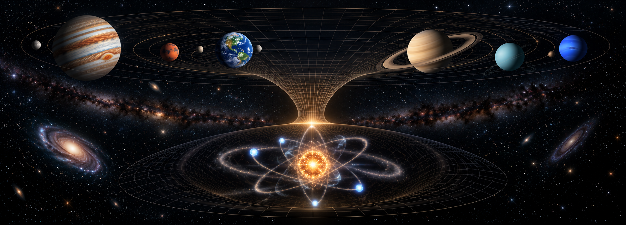
Correlating the Gravitational and Reduced Planck Constants

Jody A. Geiger

Informativity Institute

Chicago, IL USA 60607

jodygeiger@informativity.org

ORCID: 0000-0001-5389-0447

ABSTRACT

We compare Measurement Quantization (MQ) calculations of the fundamental measures with Planck’s unit expressions. The gravitational constant G, in m³ kg⁻¹ s⁻², and reduced Planck constant ħ, in J s, obey, within the MQ construction, the upper-count-limit relation 4Gp_si²=ħc³, where c is the speed of light in m s⁻¹. The momentum realization p_si is (l_fm_f)/(2t_f), in kg m s⁻¹; l_f, m_f, and t_f are the fundamental length, mass, and time measures in m, kg, and s. The Internal Frame denotes the discrete count configuration domain. Its realization in the System Frame gives a count-dependent length contraction. Paired upper-count relations reproduce the same fundamental measures. The blackbody and elementary-charge inversions are consistency calculations with their stated inputs, rather than independent verification of the framework.

Keywords: Gravitational Constant, Reduced Planck Constant, Correlation, Discrete, Informativity differential

1. INTRODUCTION

Planck’s unit expressions provide the historical context [1]. Within the MQ construction [2], the gravitational and reduced Planck realizations satisfy the following relation at the upper count limit.

4 G {p_{si}}^{2} = ħ c^{3}

(1)

The momentum realization p_si in Eq. (1) is distinct from the invariant dimensionless coefficient θ_si and its angular realization Θ_si, in radians ([2], Appx. K, P, Q, S). The numerical realization used here is p_si/(1 kg m s⁻¹) = θ_si, following the construction in [2], Appx. C, BM. The conserved quantities reviewed by Po-Ning Chen et al. [3], Sec. 4, concern general relativity at null infinity. That review is background; the MQ lower-bound construction is in [2], Appx. S. The coefficient is calibrated through [2], Appx. AD, as follows. Here α_c is the dimensionless classical fine-structure constant and n_L is the dimensionless separation count. At the Fine Structure demarcation, n_Lθ_si=276. The mixed brackets denote rounding to the nearest whole unit.

2 α_{c} = \frac{\sqrt{{θ_{si}}^{2} + 27 6^{2}} + 276}{276 (84 θ_{si} - ⌈ 42 θ_{si} ⌋)}, ​ ​ n_{L} θ_{si} = 276

(2)

Equation (2) follows by rationalizing the radical difference in [2], Appx. AD. Inverting it with the 2022 Committee on Data for Science and Technology (CODATA) inverse fine-structure input 137.035999177(21) [4] gives θ_si = 3.26239030504(25). Parentheses denote standard uncertainty propagated from the CODATA inputs in the last quoted digits, conditional on the stated MQ relations and realization assumptions. No additional uncertainty component is assigned to those assumptions in this calculation. In the supplied workbook [5], Inputs2022!A51 is hand fitted to twice the fine-structure value reconstructed in H1 from the 2022 electric permittivity and exact International System of Units (SI) constants. Its entered coefficient 3.26239030504515 differs from the exact root for that target, 3.262390305037768, by 7.38 × 10⁻¹². This is within the conditional uncertainty, but is not exact equality at every entered digit. We retain the workbook inputs for its nominal blackbody count and use the consistent 2022 calibration for the propagated MQ quantities.

The representation distinctions and their realization operators are discussed further in Measurement Quantization [2]. We use the momentum realization in dimensional equations and the invariant coefficient in the dimensionless calibration of Eq. (2). This keeps the derivation of the relation between G and ħ consistent with the numerical calculation.

The MQ construction begins with discrete expressions for gravity, the speed of light, escape velocity and Heisenberg’s uncertainty principle, whose original formulation is in [6]. Count configurations and the fundamental measures belong to the Internal Frame ([2], Appx. I, J, K). The System Frame is their continuous relational realization. The Frames mapping connects these representations; observed measures are realized in the System Frame. The resulting relations provide the MQ calculations of physical constants considered here [7].

The Informativity differential is the non-Lorentz length contraction associated with discrete count structure under the Frames mapping ([2], Appx. D). In this construction it increases as separation decreases. This count dependence is distinct from relativistic contraction; reference [8] provides historical background on relativity. A demarcation selects the count relevant to a phenomenon; it is not a common lower bound for every measurement. The upper-count limit provides the macroscopic form used below.

Upper-count-limit G and ħ are upright and finite-count measures are italic. A phenomenon-specific demarcation takes precedence. Equation (3) uses the Fine Structure demarcation, while the reduced Planck comparison uses the specified blackbody count. Where no specific count applies, the single elementary-charge default is 84.601594773245, derived in Appendix B. These dimensionless counts multiply l_f to give a length.

For a separation r = n_Ll_f, where r is the distance in m, the dimensionless Diophantine realization residual is $Q_{L} = \frac{1}{\sqrt{1 + {n_{L}}^{2}} + n_{L}}$ ([2], Appx. D). Its product Q_Ln_L controls the finite-count realizations in Eqs. (3), (13)–(15). The count is selected for the phenomenon rather than inferred from an independently measured G.

G = 2 Q_{L} n_{L} c^{3} \frac{t_{f}}{m_{f}} = 6.6738448317 (10) ​ \times ​ 1 0^{- 11} ​ m^{3} ​ k g^{- 1} ​ s^{- 2}

(3)

G = \lim_{n_{L} \to \infty} 2 Q_{L} n_{L} c^{3} \frac{t_{f}}{m_{f}} = c^{3} \frac{t_{f}}{m_{f}} = 6.6740779383 (10) ​ \times ​ 1 0^{- 11} ​ m^{3} ​ k g^{- 1} ​ s^{- 2}

(4)

Equation (3) is evaluated at the fine-structure count 84.6005456716114. Equation (4) uses the upper count limit. Both propagate the same 2022 inverse fine-structure input, 137.035999177(21), through the MQ relations, retaining their shared dependencies. The measured 2022 CODATA G = 6.67430(15) × 10⁻¹¹ m³ kg⁻¹ s⁻² is a comparison value [4], not a calibration input. The supplied spreadsheet central values agree at the displayed uncertainties; its uncertainty estimates are not adopted. Historical comparisons [9–10] remain in Table 1.

The historical values of G differ between CODATA adjustments. Within each adjustment, however, the three Planck-unit expressions in Table 1 recover the same G because the Planck measures are derived from that G and the same reduced Planck input [9–11]. The present MQ recalculation is evaluated separately; agreement of formulas sharing calibrated inputs is a consistency check.

A second comparison uses Planck’s unit expressions. Here l_p, m_p and t_p denote Planck length, mass and time in m, kg and s. Table 1 evaluates the three identities with internally consistent inputs from the 2010, 2014 and 2018 CODATA adjustments [9–11]. Treating these derived measures as independent inputs would discard their common dependencies.

Table 1. Planck-unit identities evaluated with consistent historical CODATA inputs [9–11], adapted from the comparison in [2].

CODATA^a	2010 (10^-11 m³ kg^-1 s^-2)	2014 (10^-11 m³ kg^-1 s^-2)	2018 (10^-11 m³ kg^-1 s^-2)
G=(l_p²c³)/( $ℏ$ )	6.67384(80)	6.67408(31)	6.67430(15)
G=(t_p²c⁵)/( $ℏ$ )	6.67384(80)	6.67408(31)	6.67430(15)
G=( $ℏ$ c)/(m_p²)	6.67384(80)	6.67408(31)	6.67430(15)

^a Each row recovers the recommended G for that edition. The parenthetical standard uncertainties are those of its single G input. The Planck measures and reduced Planck input retain their shared dependencies; independently propagating rounded tabular outputs does not provide a new determination of G.

The within-edition identities in Table 1 do not establish a physical discrepancy. Their former differences arose from calculations using rounded derived inputs. The following derivation compares the finite-count and upper-count MQ realizations explicitly.

The dimensional relations used below reduce to the fundamental relation l_fm_f=2p_sit_f ([2], Appx. V). Ratios such as c = l_f/t_f specify the corresponding measure conversion. Equations (5)–(7) demonstrate this reduction for Eq. (1) at the upper count limit.

By example, consider Eq. (1). Substituting the momentum realization defined above, the upper-count-limit solution G=(l_f)/(t_f)³(t_f)/(m_f) ([2], Appx. F), and ħ=(l_f²m_f)/(t_f) ([2], Appx. B), gives

4 (\frac{l_{f}^{3}}{t_{f}^{3}} \frac{t_{f}}{m_{f}}) {(\frac{l_{f} m_{f}}{2 t_{f}})}^{2} = (\frac{l_{f}^{2} m_{f}}{t_{f}}) c^{3}

(5)

4 \frac{l_{f}^{3}}{t_{f}^{3}} \frac{t_{f}}{m_{f}} \frac{l_{f}^{2} m_{f}^{2}}{4 t_{f}^{2}} = \frac{l_{f}^{2} m_{f}}{t_{f}} \frac{l_{f}^{3}}{t_{f}^{3}}

(6)

1 = 1

(7)

2. METHODS

We apply the MQ count construction to classical relations for gravitational curvature, the speed of light, escape velocity and Heisenberg’s uncertainty principle. These comparisons extend the applications in [2, 7, 12–16] and distinguish finite-count inputs from the upper count limit.

The discreteness and countability of measure are premises of the MQ construction used here. The introductory paper Measurement Quantization [2] develops these premises and their proposed measurement applications. Its appendices supply the mathematical context for this paper. A preprint is available in Online Resources.

https://www.researchgate.net/publication/361148724_OnlineResources

The supplementary spreadsheets described in [2] provide calculation implementations. Suppl. 1 covers the introductory paper and its appendices; Suppl. 2 is described as covering this paper and other MQ applications [2, 7, 12–16]. The supplied workbook [5] additionally fixes the nominal blackbody-count implementation examined here. Agreement with calibrated inputs is assessed as consistency, with independent source measurements retained for comparison.

3. RESULTS

The count most relevant to a phenomenon is its demarcation. Equation (3) uses the Fine Structure demarcation. Equations (22)–(24) give the reduced Planck inversion; Eq. (23) records the separate nominal workbook count 84.6005393909226. Appendix B supplies the elementary-charge default when no more specific demarcation is available. Neither inversion is a prediction from first principles.

The component measures must refer to the stated demarcation. At the upper count limit, the recalculated quantities are G=6.6740779383(10) × 10^-11 m³ kg^-1 s^-2 and ħ=1.0545349844417293(56) × 10^-34 J s. Their uncertainties propagate the shared 2022 input chain. Inserting these paired quantities into Eqs. (8)–(12) gives the same fundamental measures. This is algebraic consistency under a common realization. The exact SI value $ℏ$ = (h)/(2π) [4] is used for the finite-count comparison. Here h is Planck’s constant and π is the circle constant. The different upper-count quantity is an MQ realization; these equations do not establish a distance variation of the SI defining constant. The source spreadsheet and its nonzero uncertainties for exact SI constants are retained only in the calculation record for comparison.

1. Calculations

To demonstrate the relation between G and ħ, we begin with expressions for the fundamental measures ([2], Appx. W). These are compared with Planck’s unit expressions in Eqs. (8)–(10). Here both G and ħ are evaluated at the upper count limit, and p_si is the momentum realization.

\frac{2 G p_{si}}{c^{3}} = \sqrt{\frac{ħ G}{c^{3}}}

(8)

\frac{2 G p_{si}}{c^{4}} = \sqrt{\frac{ħ G}{c^{5}}}

(9)

\frac{2 p_{si}}{c} = \sqrt{\frac{ħ c}{G}}

(10)

Each expression can be reduced to,

4 G {p_{si}}^{2} = ħ c^{3}

(11)

Given that G=(c³t_f)/(m_f) ([2], Appx. F) then,

ħ = 2 p_{si} l_{f} = \frac{{l_{f}}^{2} m_{f}}{t_{f}}

(12)

Equation (12) relates the upper-count quantities and uses the fundamental relation established above. The angular-momentum construction is discussed in [2], Appx. R. Equations (20)–(21) give the fundamental measures from the 2022 calibration, with the momentum realization used in dimensional expressions.

The finite-count forms follow by retaining the factor 2Q_Ln_L in G and its reciprocal in $ℏ$ ([2], Appx. D, L, M). This is why Eq. (1) cannot be used unchanged with an arbitrary finite-count pair.

ℏ = \frac{p_{si} l_{f}}{Q_{L} n_{L}}

(13)

G = \frac{Q_{L} n_{L} l_{f} c^{3}}{p_{si}} = 2 Q_{L} n_{L} {(\frac{l_{f}}{t_{f}})}^{3} \frac{t_{f}}{m_{f}}

(14)

For positive n_L, 0 < Q_Ln_L < 1/2. The product approaches one half at the upper count limit. At finite count, Eqs. (13)–(14) require the divisor (2Q_Ln_L)² in Eq. (15). Substitution gives Eqs. (16)–(18); cancellation is valid because p_si and Q_Ln_L are positive. The fundamental relation therefore follows before taking the limit.

ℏ = \frac{4 {p_{si}}^{2} G}{c^{3} {(2 Q_{L} n_{L})}^{2}}

(15)

\frac{p_{si} l_{f}}{Q_{L} n_{L}} = \frac{4 {p_{si}}^{2}}{c^{3} {(2 Q_{L} n_{L})}^{2}} (2 Q_{L} n_{L} c^{3} \frac{t_{f}}{m_{f}})

(16)

p_{si} l_{f} = 2 {p_{si}}^{2} \frac{t_{f}}{m_{f}}

(17)

l_{f} m_{f} = 2 p_{si} t_{f}

(18)

The count limit of Q_Ln_L is ([2], Appx. D),

\lim_{n_{L} \to \infty} (Q_{L} n_{L}) = \frac{1}{2}

(19)

Equation (18) gives the fundamental relation. Equation (19) then recovers Eq. (1) from Eq. (15) at the upper count limit. At a selected separation, the fractional attenuation of G relative to its upper-count value is 1 − 2Q_Ln_L. Table 2 evaluates this dimensionless fraction using Eqs. (3–4).

Table 2. Fractional attenuation 1 − 2Q_Ln_L at selected separations, calculated from Eqs. (3)–(4), following the comparison in [2].

	84.6005394 l_f	500 l_f	10,000 l_f	a₀ a	1 m	13.794 Gly
Fraction	3.49272 × 10⁻⁵	9.99998 × 10⁻⁷	2.50 × 10⁻⁹	< 10⁻³⁰ b	< 10⁻³⁰ b	< 10⁻³⁰ b

^a Describes the distance associated with the ground state orbital of an atom.

^b Exceeds the physical significance of the source measures.

2. Numerical Comparisons

Table 2 shows that the finite-count factor becomes negligible at ordinary laboratory distances, while it remains relevant at counts near the electromagnetic demarcations. The Planck-unit comparison therefore must specify whether each constant is evaluated at finite count or at the upper count limit.

Table 3 uses [2], Appx. BM, with the consistent 2022 calibration from Eq. (2). Here m_e is the electron mass in kg, a₀ the Bohr radius in m, and α_p^-1 the dimensionless Planck-like inverse fine-structure coupling. Their product is evaluated as m_ea₀=( $ℏ$ α_c^-1)/(c) to retain the CODATA dependency. The same classical inverse fine-structure input determines θ_si; independent propagation of these shared quantities would count that input more than once.

m_{f} = \frac{2 p_{si}}{c}, ​ ​ {α_{p}}^{- 1} = 84 θ_{si} - ⌈ 42 θ_{si} ⌋

(20)

l_{f} = \frac{m_{e} a_{0}}{{α_{p}}^{- 1} m_{f}}, ​ ​ t_{f} = \frac{l_{f}}{c}

(21)

The first row of Table 3 evaluates the usual Planck expressions with exact SI $ℏ$ and the MQ upper-count G; the second gives the fundamental measures from Eqs. (20)–(21). The momentum column reports $\sqrt{\frac{ℏ c^{3}}{4 G}}$ for the first row and p_si for the second. It does not label a momentum as an angle. The blackbody count is retained at its author-specified working precision.

Table 3. Updated Planck and fundamental measures, adapted from [15], with 2022 CODATA comparison [4].

Input	n_L	Momentum (kg m s⁻¹)	Length (10⁻³⁵ m)	Time (10⁻⁴⁴ s)	Mass (10⁻⁸ kg)
$ℏ$	84.6005393909226	3.26244727955(25)	1.61622813686(12)	5.39115676105(41)	2.17647054987(17)
ħ	∞	3.26239030504(25)	1.61619991148(12)	5.39106261131(41)	2.17643254057(17)
2022 [4]	—	—	1.616255(18)	5.391247(60)	2.176434(24)

Parentheses in the first two rows are conditional standard uncertainties propagated from the single 2022 inverse fine-structure input. No additional uncertainty is assigned to the MQ model or realization assumptions beyond that input propagation. The blackbody count in the first row is the nominal workbook reference [5], 2022Calcs!J86; it does not set that row’s other numerical columns, which use exact SI $ℏ$ and the consistent MQ upper-count G. The retained working count is not a 15-digit measurement.

The last row uses the 2022 CODATA measured G and exact SI $ℏ$ [4]. The first two rows share the calculated MQ upper-count G and are not independent tests. Their first-row Planck expressions mix exact SI $ℏ$ with upper-count G, whereas the second row uses the paired upper-count quantities of Eqs. (8)–(12).

4. DISCUSSION

The invariant dimensionless coefficient θ_si and the distinct momentum realization p_si provide, within the MQ construction, a way to describe the relation between the gravitational and reduced Planck constants. The upper-count-limit identity in Eq. (1) and the finite-count identity in Eq. (15) preserve their respective realizations, with the latter accounting for the Informativity differential.

Within the MQ relations, the finite-count effect is greatest at small separations and falls rapidly toward the upper count limit. At the Bohr-radius example in Table 2, it is smaller than 10⁻³⁰ as a fraction. The relevant demarcation still depends on the phenomenon; laboratory separation alone does not determine the count appropriate to every constant.

Within the MQ construction, the finite-count relations affect G and $ℏ$ in reciprocal ways. Ordinary macroscopic G measurements are compared with the upper-count limit, whereas the reduced Planck comparison uses the selected finite-count realization. The calculated upper-count G in Eq. (4) is 1.48 combined standard uncertainties below the 2022 CODATA recommended G [4]. This comparison combines the propagated input uncertainty with the CODATA G uncertainty; G was not used for the MQ calibration. CODATA determines G separately from its other adjusted constants and retains expanded uncertainties because its experimental inputs are inconsistent [4], Secs. XIV–XV. The comparison therefore supplies a numerical consistency test, not proof of the MQ interpretation.

For the reduced Planck constant, the relevant count is the blackbody demarcation ([2], Appx. AB). The supplied calculation [5], 2022Calcs!J86, evaluates Eq. (22) using p_si from 2022Calcs!F19 and l_f and $ℏ$ from Inputs2022!E10 and B6. Its stored result, 84.600539390922592, rounds to the working value in Eq. (23). This repeats the reduced Planck input through the stated nominal MQ realization; it is not a prediction from first principles.

n_{L} = p_{si} l_{f} \sqrt{\frac{1}{ℏ (ℏ - 2 p_{si} l_{f})}}

(22)

n_{L} = 84.6005393909226

(23)

Using Eq. (12), the inversion can be written with upright ħ at the upper count limit and italic $ℏ$ at the blackbody demarcation. The workbook obtains p_si = 3.2623903050451251 kg m s⁻¹ through F19 = (l_fm_f)/(2t_f), with its measures from [2], Appx. BM, calculated from the hand-fitted coefficient in Inputs2022!A51 and the printed 2022 electron-mass and Bohr-radius inputs [5]. Native Excel reproduces J86 exactly. The count 84.6005456716114 follows instead from the consistent fine-structure calibration and exact Bohr-product dependency used for Table 3. Both calculations use the same relation in [2], Appx. AD; their different nominal inputs explain the numerical discrepancy.

The denominator subtracts two nearby quantities, making the count sensitive to numerical precision. Inputs2022!B6 stores text evaluated with π = 3.14159265358979; ordinary Excel arithmetic then converts the input strings to numeric values. High-precision evaluation of the same nominal inputs from [2], Appx. BM, with exact (h)/(2π) gives 84.6005393994101, differing by 8.49 × 10⁻⁹. We retain 84.6005393909226 as the specified workbook working value, without assigning physical significance to all displayed digits or adopting its historical uncertainty estimate.

n_{L} = \frac{ℏ}{2} \sqrt{\frac{1}{ℏ (ℏ - ℏ)}}

(24)

Expressions containing both G and ħ require a consistent realization. With the paired upper-count quantities, Eqs. (8)–(12) yield the fundamental measures. Combining exact SI $ℏ$ with upper-count G instead gives the first-row Planck measures in Table 3. This distinction is algebraic and does not independently establish the physical interpretation. At a separation of one meter, the computed fractional attenuation of G is below 10⁻³⁰, as Table 2 shows.

5. APPENDICES

APPENDIX A: TERMS

Source term and measure definitions are given in Measurement Quantization [2], Appx. K, T, W.

The coefficient and its momentum and angular realizations are distinguished in the introduction. References [17–19] concern X-ray polarization, parametric down-conversion and wave mixing; they are distinct from the fine-structure calibration used here. We do not infer an independent angular or momentum measurement from those citations. The general-relativistic conserved-quantity background remains in [3], Sec. 4.

The speed of light introduced above satisfies c = (n_Ll_f)/(n_Tt_f). Here n_T is the dimensionless time count, with n_L=n_T for this conversion. The exact SI value is 299,792,458 m s⁻¹ [4]; the one-unit reference uses n_L=n_T=1.

The upper-count and finite-count values of G, with conditional propagated 2022 uncertainties, are given in Eqs. (3)–(4). The nominal upper-count result is 6.67407793827854 × 10⁻¹¹ m³ kg⁻¹ s⁻². The finite-count value depends on the phenomenon-specific demarcation.

The fundamental measures introduced in the abstract are evaluated in Table 3. Their distinction from the Planck measures follows from the input realizations described beside that table.

The Planck measures introduced before Table 1 are evaluated with their stated G and $ℏ$ inputs; their units remain m, kg and s.

The length and time counts are used above; n_M denotes the dimensionless count of the fundamental mass measure. Their physical interpretation follows the MQ count construction in [2].

The separation count introduced above describes a change in position relative to an observer; its reference must be specified when applying the finite-count equations.

A separation measured from a center of mass uses the same count notation with that reference specified. It does not introduce a second independent count definition.

n_Lc describes the count of l_f representative of a change in position of light measured with respect to the observer’s frame of reference.

The metric differential is the normalization mismatch when a conserved discrete count configuration is realized continuously under the Frames mapping. It is a representation mismatch, distinct from the physical length contraction described by the Informativity differential.

n_θ is the whole-unit count associated with half of the interaction count after the metric differential is accounted for. The mixed brackets ⌊x⌉ denote rounding to the nearest whole-unit value, with x denoting the real-valued argument, giving ⌊(84.60055)/(2)⌉=42.

The ordinary brackets ⌊x⌋ and ⌈x⌉ denote floor and ceiling, respectively; the mixed pair used above denotes the MQ nearest-whole-unit convention.

The residual introduced before Eq. (3) is used throughout the finite-count derivation. Its limiting product with the count is given by Eq. (19).

The product Q_Ln_L supplies the finite-count factors in Eqs. (13)–(15); the associated length contraction is the Informativity differential described in the introduction.

The finite-count reduced Planck constant uses the exact SI value (h)/(2π) = 1.054571817646156… × 10⁻³⁴ J s [4]. Its upper-count MQ realization is ħ=1.0545349844417293(56) × 10^-34 J s, with conditional propagated input uncertainty. Exactness of the SI input does not make an inferred demarcation an independently predicted or exact count.

The electron-mass input in Eq. (21) belongs to the 2022 CODATA adjustment [4]; its product with the Bohr radius is evaluated through the shared fine-structure dependency.

The Bohr-radius input in Eq. (21) belongs to the same adjustment [4]. The product treatment above retains its dependence on the electron mass and fine-structure input.

The dimensionless fundamental inverse coupling α_f^-1 = 42θ_si belongs to the Internal Frame construction. The Planck-like coupling in Eq. (20) and classical coupling in Eq. (2) describe distinct System Frame realizations; their difference retains the finite-count factor [2].

The historical γ construction is superseded for this calculation by the fundamental electromagnetic parameter γ_F. Its dimensionless configuration representation and SI charge normalization are specified in Appendix B. The older γ approximation is not used in the elementary-charge inversion.

APPENDIX B ELECTROMAGNETIC DEMARCATION FROM ELEMENTARY CHARGE

The supplied fundamental construction replaces the older γ approximation. The default is used only in the absence of an unambiguous phenomenon-specific count. The quantities e_f, e_p and e_c are the fundamental, Planck-like and classical charge realizations in coulombs; n_e is a charge-valued intermediate. The dimensionless residual Q_{n_θ} differs from the integer interaction count in Appendix A. SI numerical coefficients below make the Frames mapping explicit.

\frac{e_{f}}{1 ​ C} = \frac{\frac{l_{f}}{1 ​ m} {(\frac{c}{1 ​ m ​ s^{- 1}})}^{2}}{4 (θ_{si} - 1)}

(B.1)

Q_{n_{θ}} = 42 θ_{si} - ⌈ 42 θ_{si} ⌋, ​ ​ n_{e} = (84 \frac{e_{f}}{1 ​ C} - ⌈ 42 \frac{e_{f}}{1 ​ C} ⌋) ​ (1 ​ C)

(B.2)

e_{p} = \frac{n_{e}}{84 + \frac{42}{277 - 3 Q_{n_{θ}} - 7 {Q_{n_{θ}}}^{2} - 14 {Q_{n_{θ}}}^{3}}}

(B.3)

Equations (25)–(27) follow the author-supplied charge construction. The polynomial uses the residual Q_{n_θ}, resolving the older source notation. Equation (28) defines the fundamental electromagnetic parameter in normalized dimensionless form. Multiplication by (1 C)² recovers its charge-squared SI realization.

γ_{F} = {α_{p}}^{- 1} {({(Q_{L} n_{L})}^{2} \frac{e_{p}}{1 ​ C})}^{2}

(B.4)

e_{c} = 2 Q_{L} n_{L} e_{p} = \frac{2 ​ C}{Q_{L} n_{L}} \sqrt{\frac{γ_{F}}{{α_{p}}^{- 1}}}

(B.5)

Let K denote the dimensionless product Q_Ln_L in this inversion. The exact elementary-charge input is e_c = 1.602176634 × 10⁻¹⁹ C [4]. It fixes the count through e_p; a finite positive count requires 0 < K < 1/2.

K = Q_{L} n_{L} = \frac{e_{c}}{2 e_{p}}, ​ ​ Q_{L} = \frac{1}{\sqrt{1 + {n_{L}}^{2}} + n_{L}}

(B.6)

Multiplying the count relation gives $K + {n_{L}}^{2} = n_{L} \sqrt{1 + {n_{L}}^{2}}$ . Squaring and cancelling the fourth-power terms yields n_L²(1-2K)=K². Selecting the positive root gives the explicit elementary-charge inversion.

n_{L} = \frac{K}{\sqrt{1 - 2 K}} = \frac{e_{c}}{2 e_{p} \sqrt{1 - \frac{e_{c}}{e_{p}}}}

(B.7)

n_{L} = 84.60159 (23)

(B.8)

The single working default is 84.601594773245 from the consistent 2022 input chain. Equation (32) gives its conditional propagated uncertainty. The supplied printed-input construction gives 84.601607423665, consistent at this uncertainty, and is retained only as a source comparison. The exact charge is used for the inversion, so recovering it is a consistency calculation. The fundamental construction removes the old measured-γ route, but this numerical SI realization still inherits its stated calibration inputs; it is not an independent verification of those inputs.

STATEMENTS AND DECLARATIONS

The author has no relevant financial or non-financial interests to disclose.

The author has no competing interests to declare that are relevant to the content of this article.

DATA AVAILABILITY

The source paper describes electronic supplementary calculations [2]. The workbook [5] supplies the nominal calculation traced in the blackbody-count discussion; the revision record preserves its input cells, formula dependencies and precision comparison.

REFERENCES

[1] M. Planck, Über irreversible Strahlungsvorgänge, Sitzungsberichte der Königlich Preußischen Akademie der Wissenschaften zu, Berlin, 5, p. 480 (1899).

[2] J.A. Geiger: Measurement Quantization, International Journal of Geometric Methods in Modern Physics 20(4), 2350069 (2023), CC BY 4.0, doi:10.1142/S021988782350069X.

[3] Po-Ning Chen, Mu-Tao Wang, Ye-Kai Wang, Shing-Tung Yau, Conserved quantities in general relativity -- the view from null infinity (Apr. 8, 2022), doi:10.48550/arXiv.2204.04010.

[4] P. J. Mohr, D. B. Newell, B. N. Taylor, and E. Tiesinga, CODATA recommended values of the fundamental physical constants: 2022, Reviews of Modern Physics 97, 025002 (2025), Tables XXXII–XXXIII and Secs. XIV–XV, doi:10.1103/RevModPhys.97.025002.

[5] J. A. Geiger, MQSigma.xlsx, supplied calculation workbook, Inputs2022 and 2022Calcs worksheets, snapshot supplied 13 October 2026. The blackbody-count calculation is in 2022Calcs!J86.

[6] Heisenberg, W., Über den anschaulichen Inhalt der quantentheoretischen Kinematik und Mechanik, Zeitschrift für Physik, 43 (3–4): 172–198 (1927), Bibcode:1927ZPhy.43.172H, doi:10.1007/BF01397280, S2CID 122763326.

[7] J.A. Geiger: Measurement Quantization Describes the Physical Constants, International Journal of Theoretical and Mathematical Physics, 11(1), pp. 29-59 (Jan 2021), doi:10.5923/j.ijtmp.20211101.03.

[8] Albert Einstein, The Collected Papers of Albert Einstein, Vol. 6, The Berlin Years: Writings, 1914–1917 (English translation of selected texts), Princeton University Press (1997). Volume information: https://www.einstein.caltech.edu/what-we-do/published-volumes/volume-6

[9] P. J. Mohr, B. N. Taylor, and D. B. Newell, CODATA recommended values of the fundamental physical constants: 2010, Reviews of Modern Physics 84, 1527–1605 (2012), doi:10.1103/RevModPhys.84.1527.

[10] P. J. Mohr, D. B. Newell, and B. N. Taylor, CODATA recommended values of the fundamental physical constants: 2014, Reviews of Modern Physics 88, 035009 (2016), doi:10.1103/RevModPhys.88.035009.

[11] E. Tiesinga, P. J. Mohr, D. B. Newell, and B. N. Taylor, CODATA recommended values of the fundamental physical constants: 2018, Reviews of Modern Physics 93, 025010 (2021), doi:10.1103/RevModPhys.93.025010.

[12] J.A. Geiger: Measurement Quantization Unites Classical and Quantum Physics, Journal of High Energy Physics Gravitation and Cosmology. Vol. 4, No. 2, 262–311 (Apr 2018), doi:10.4236/jhepgc.2018.42019.

[13] J.A. Geiger: Quantum Model of Gravity Unifies Relativistic Effects, Describes Inflation/Expansion Transition, Matches CMB Data, Journal of High Energy Physics Gravitation and Cosmology. Vol. 4, No. 4 (Oct 2018), doi:10.4236/jhepgc.2018.44038.

[14] J.A. Geiger: Measurement Quantization Describes Galactic Rotational Velocities, Obviates Dark Matter Conjecture, Journal of High Energy Physics Gravitation and Cosmology. Vol. 5, No. 2 (Apr 2019), doi:10.4236/jhepgc.2019.52028.

[15] J.A. Geiger: Physical Significance of Measure, Journal of High Energy Physics Gravitation and Cosmology. Vol. 6, No. 1 (Jan 2020), CC BY 4.0, doi:10.4236/jhepgc.2020.61008.

[16] J.A. Geiger: Measurement Quantization Describes History of Universe – Quantum Inflation, Transition to Expansion, CMB Power Spectrum, Journal of High Energy Physics Gravitation and Cosmology. Vol. 6, No. 2 (Apr 2020), doi:10.4236/jhepgc.2020.62015.

[17] S. Shwartz and S. E. Harris, Polarization Entangled Photons at X-Ray Energies, Phys. Rev. Lett. 106, 080501 (2011), arXiv: 1012.3499, doi:10.1103/PhysRevLett.106.080501.

[18] S. Shwartz, R. N. Coffee, J. M. Feldkamp, et. al., X-ray Parametric Down-Conversion in the Langevin Regime, Physical Review Letters, 109, 013602 (July 6, 2012), doi:10.1103/PhysRevLett.109.013602.

[19] T. E. Glover et al., X-ray and optical wave mixing, Nature, 488, 7413, 603–608 (2012), doi:10.1038/nature11340.