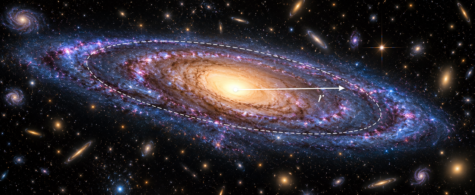
Bounds to Baryonic Density

Jody A. Geiger

Informativity Institute

Chicago, IL USA 60605

jodygeiger@informativity.org

ORCID: 0000-0001-5389-0447

ABSTRACT

We investigate how geometric count relations in Measurement Quantization impose bounds on gravitational mass relative to radial distance. Requiring classical escape speed to remain below the speed of light yields a mass-to-length count ratio strictly below one-half under the upper-count gravitational normalization. The central dimensionless transform connects this ratio to matched inertial and gravitational contraction factors using only counts of fundamental measures. It links the discrete Internal Frame to observable geometry in the System Frame through the Frames mapping. We then examine a galactic bound-speed prescription that maps an adopted Milky Way modeled velocity to an effective velocity. Across 84 samples spanning 1,000–84,000 light-years, the velocity residuals have a population standard deviation of 1.394 km/s. This comparison illustrates the prescription without providing independent empirical validation. The principal result is a conditional geometric bound on mass relative to length; a density bound additionally requires a specified volume and mass distribution.

Keywords: Baryonic Density, Mass Bound, Discrete Bound, Mass, Measure

1. INTRODUCTION

Using the Measurement Quantization (MQ) approach to classical expressions [1], this paper addresses bounds on length and mass counts in the Internal Frame and their interpretation through the System Frame. The discussion retains the classical upper-count normalization when reducing the gravitational relation to a ratio of counts.

Let l_f, m_f and t_f denote the fundamental measures of length, mass and time, with units m, kg and s in the International System of Units (SI). Their dimensionless discrete counts, with positive length and time counts in the speed normalization, are n_L, n_M and n_T. The symbol c denotes the speed of light. The relation

c = \frac{n_{L} l_{f}}{n_{T} t_{f}}

reduces to the fundamental speed when the length and time counts are equal. The reciprocal fundamental time supplies the fixed count rate of this construction. Planck [2] supplies the historical context of natural units, rather than a measurement of this MQ rate. Our principal bound concerns

\frac{n_{M}}{n_{L}}

, whose upper limit is one-half in the subluminal classical escape-speed comparison. A frequency is a count rate, not a dimensionless count.

This investigation builds on Measurement Quantization [1], where gravitational expressions, the speed of light, escape velocity and Heisenberg’s uncertainty principle [3] motivate the fundamental-measure construction. Discrete and countable measure in the Internal Frame and its non-discrete System Frame realization are MQ premises ([1], Appx. I, J). Comparisons with values recommended by the Committee on Data of the International Science Council (CODATA) in [1], Table 2, must distinguish measured inputs from derived quantities; reproducing an input or an algebraic consequence of it is internal consistency rather than independent evidence.

The spatial ratio bound follows from (13)–(15); the fixed count rate in (6) supplies a separate normalization. The effective mass and effective velocity ([1], Appx. AH, AI) are realized model quantities. The galactic example uses a curve attributed to McGaugh’s Milky Way model [4] as input. Its residual statistics and the limits of that comparison are specified below.

2. METHODS

We reduce classical expressions using MQ fundamental measures and counts, retaining their stated upper-count domain. Related applications appear in [1, 5–10]. These publications describe the MQ program; their existence does not establish the empirical validity of every application.

The construction and its proposed physical interpretation are developed in Measurement Quantization [1]. Here the cancellation of fundamental units is a mathematical result conditional on those premises. A claim that nature realizes discrete counts additionally requires observations capable of distinguishing that interpretation from the classical descriptions used to construct the relation.

https://www.researchgate.net/publication/361148724_OnlineResources

The Online Resources link identifies supplementary calculations associated with the MQ publications. The numerical comparison in this paper can be reproduced from the four series embedded in Fig. 1. Those series permit a check of the velocity mapping and its residuals, but do not specify the original model selection, digitization or interpolation procedure.

3. RESULTS

The count formulation allows the escape-speed expression to be reduced without retaining the fundamental-unit factors. Here v denotes escape speed, and G is the upright upper-count gravitational constant, with units m³ kg⁻¹ s⁻² and normalization

G = \frac{c^{3} t_{f}}{m_{f}}

. In (2–4), n_L is the radial length count and n_M the enclosed mass count. Equation (1) is the formal one-mass, one-length starting expression ([1], Appx. AV). It lies outside the subluminal bound. Equations (2–4) introduce the general counts and use l_f=ct_f to obtain the dimensionless ratio.

| v | = \sqrt{\frac{2 G m_{f}}{l_{f}}}

,

(1)

v^{2} = \frac{2 G n_{M} m_{f}}{n_{L} l_{f}} = \frac{2 n_{M} c^{3} t_{f}}{n_{L} l_{f}}

,

(2)

v^{2} = \frac{2 n_{M} c^{2}}{n_{L}}

,

(3)

\frac{v^{2}}{c^{2}} = 2 \frac{n_{M}}{n_{L}}

.

(4)

To connect this result with inertial contraction, n_Lc denotes the count of light-displacement lengths over the same positive comparison interval. The left side of (5) uses the displacement count in the inertial comparison; its right side uses the radial count in the gravitational comparison. Their identification is the matched comparison developed in [1], Appx. AW, not an automatic identification of every displacement with every radius.

\frac{n_{L}^{2}}{n_{L c}^{2}} = 2 \frac{n_{M}}{n_{L}}

.

(5)

Equation (5) is the central geometric transform in this argument. The factors of l_f, m_f and t_f cancel, leaving only counts in the matched inertial and gravitational contraction comparison. For a nondegenerate subluminal comparison, the common ratio is below unity and the radial count is positive. The derivation establishes this conditional relation; cancellation of units alone does not prove that nature implements the assumed discrete geometry.

The fixed count-rate normalization can be expressed independently of the spatial bound ([1], Appx. O). Equation (6) combines the length count rate obtained from c with the mass count rate obtained from the upper-count gravitational normalization. Each member has units s−1.

\frac{c}{l_{f}} = \frac{c^{3}}{G m_{f}} = \frac{1}{t_{f}}

,

(6)

Equation (6) follows from the speed normalization and the upper-count gravitational relation. Equation (7) retains the factorization used to obtain that gravitational relation ([1], Appx. F).

G = {(\frac{l_{f}}{t_{f}})}^{3} \frac{t_{f}}{m_{f}}

.

(7)

The speed formed from length and time appears cubed in (7), whereas the time-to-mass factor has units s kg−1. Neither is a frequency. Their product has the dimensions of the gravitational constant. Combining (7) with the speed normalization gives the common fixed count rate in (6), without identifying counts with rates.

Equation (8) retains the arithmetic identities used to illustrate equal unit-normalized values. These identities do not equate quantities of different dimensions or derive a physical count-rate bound.

1^{1} = 1^{3}, \sqrt[1]{1} = \sqrt[3]{1}

.

(8)

1. Count Bound Relation of Mass to Length

The function marker f in (9)–(12) denotes evaluation of the displayed count ratio. Equation (9) compares equal counts. Equations (10)–(12) compare rates with the same units, using the fixed rate in (6) and a selected one-count-per-second rate. The common units cancel, so the normalized ratios are dimensionless.

f (\frac{n_{M}}{n_{L}}) = \frac{1}{1} = 1

(9)

f (\frac{n_{M}}{n_{L}}) = \frac{1 / t_{f}}{1 / t_{f}} = 1

(10)

f (\frac{n_{M}}{n_{L}}) = \frac{1 ​ s^{- 1}}{1 / t_{f}} = \frac{t_{f}}{1 ​ s}

(11)

f (\frac{n_{M}}{n_{L}}) = \frac{1 / t_{f}}{1 ​ s^{- 1}} = \frac{1 ​ s}{t_{f}}

(12)

The equal-count and equal-rate examples (9) and (10) give unity. Equation (11) is a selected rate ratio, not a universal lower bound. The reversed example (12) is arithmetic outside the subluminal domain. To obtain the physical upper condition, we require escape speed below c in the classical upper-count gravitational expression ([1], Appx. G). Here M is enclosed dimensional mass, r is radial distance, and v_escape distinguishes escape speed from the later effective velocity.

v_{escape} = \sqrt{\frac{2 G M}{r}}

,

(13)

c > v_{escape} = c \sqrt{\frac{2 n_{M}}{n_{L}}}

,

(14)

\frac{n_{M}}{n_{L}} < \frac{1}{2}

.

(15)

Equation (15) is a necessary count-ratio condition for the adopted subluminal classical escape-speed comparison, with nonnegative mass counts and positive radial counts. It is not a general bound on density, which also requires a spatial volume and mass distribution. At finite interaction counts, the gravitational coupling retains the Informativity differential, the count-dependent normalization describing non-Lorentz length contraction of realized separations, distinct from curvature. A finite-count threshold must be derived from that coupling rather than identified with the upper-count result.

2. Modeled Velocity Comparison

The galactic example applies a bounded count prescription to realized gravitational motion. We distinguish the Internal Frame count construction from the System Frame quantities used in the velocity comparison. The prescription is developed in two steps.

First, the bounded count construction supplies the effective mass

M_e and the effective velocity v_e, with mass and speed units respectively ([1], Appx. AH, AI). They are the realized System Frame quantities used in this comparison. The fixed rate in (6) provides the fundamental normalization; it is not an equation asserting that a dimensionless count exceeds a frequency.

The baseline bound speed v_bc in (16) uses the count-based escape-speed expression ([1], Appx. AF). Its last equality selects

\frac{n_{M}}{n_{L}} = \frac{m_{f}}{1 k g}

. The ratio

\frac{m_{f}}{1 k g}

extracts the numerical value of the dimensional mass in kilograms; m_f retains its mass dimension. The reference mass remains one kilogram when units are converted. This selected numerical normalization is an additional prescription, not a consequence of the upper inequality alone.

v_{b c} = c \sqrt{\frac{2 n_{M}}{n_{L}}} = c \sqrt{2 \frac{m_{f}}{1 ​ kg}}

.

(16)

The invariant coefficient θ_si is dimensionless. Equation (17) uses it to obtain the realized bound speed v_b from the baseline speed. It is the scalar factor used in this prescription, rather than a dimensionful expansion rate. The metric differential characterizes the mismatch between discrete count structure and continuous realization under the Frames mapping ([1], Appx. T). This representation mismatch is not a physical deformation in itself.

v_{b} = θ_{s i} c \sqrt{2 \frac{m_{f}}{1 ​ kg}}

.

(17)

The bound mass M_b has mass units, and R is the radius of the bound system, with R=n_Ll_f. Equation (18) uses the circular-speed form to define the mass associated with the bound speed. Solving gives (19), using the same upper-count gravitational normalization ([1], Appx. AG). This spherical enclosed-mass form is part of the bound prescription; it is not the calculation of a flattened galactic disk’s field.

θ_{s i} c \sqrt{2 \frac{m_{f}}{1 ​ kg}} = \sqrt{\frac{G M_{b}}{R}}

,

(18)

M_{b} = \frac{R v_{b}^{2}}{G} = 2 θ_{s i}^{2} n_{L} m_{f} \frac{m_{f}}{1 ​ kg}

.

(19)

Let v_m denote the modeled speed from the adopted mass distribution. Equation (20) defines its relative difference from v_b. The differential is dimensionless, and the bound speed must be nonzero. The baseline speed in (16) and the realized bound speed in (17) remain distinct. The notation Δ_{f(v_m)} labels this modeled-speed differential.

Δ_{f (v_{m})} = \frac{(v_{m} - v_{b})}{v_{b}}

.

(20)

Equation (21) gives the effective velocity from the modeled and bound speeds ([1], Appx. AK). Its second equality is the exact expansion of the first. A real nonnegative effective speed requires the modeled speed to be at least half the positive bound speed.

v_{e}^{2} = v_{b}^{2} (2 \frac{v_{m}}{v_{b}} - 1) = 2 v_{m} v_{b} - v_{b}^{2}

.

(21)

We retain v_m as the modeled input rather than substituting an independently measured effective-mass profile. Equation (21) does not require the effective speed to equal that input at every radius. If equality is imposed, its quadratic reduction gives equality with the bound speed as well. This is a fixed-point condition, not a general solution for an arbitrary velocity profile.

A difference between the effective and modeled speeds is the residual evaluated in the comparison shown in Fig. 1. Equality of these speeds does not by itself establish a minimum-energy trajectory.
The modeled speed remains correlated with the adopted enclosed-mass profile. The bound prescription must be evaluated against that profile rather than replacing the profile with the fixed-point condition.

McGaugh [4] constructs Milky Way rotation curves from a baryonic disk, bulge and gas model with a specified interpolation for modified Newtonian dynamics (MOND). Its modeled circular speed is distinct from the Newtonian baryonic speed. Figure 1 retains an adopted curve attributed to that work; the particular scale length and interpolation choice used in the embedded series are not specified. Equation (21) takes this adopted modeled curve as input. The comparison therefore cannot be treated as a fresh prediction from the baryonic mass distribution alone.

The embedded series contain 84 samples at 1,000-light-year spacing from 1,000 to 84,000 light-years. With bound speed 204.0535823631963 km/s, (21) reproduces the effective series to numerical rounding. For effective minus modeled speed, the population standard deviation is 1.394009 km/s, the mean is −1.090618 km/s, and the root-mean-square residual is 1.769946 km/s. These are unweighted curve-comparison statistics, not measurement uncertainties or an independent goodness-of-fit test. The plotted zero-radius origin is illustrative and excluded because it does not satisfy the real-speed domain of (21).

Figure 1. Milky Way velocities. Classical curve blue, modeled curve green, effective curve red, and bound speed purple. Radius is in thousands of light-years; speed is in km/s. — **Fig. 1.** Adopted modeled curve (green) attributed to [4], mapped effective curve (red), bound speed (purple) and retained classical curve (blue). Reprinted from [1], Fig. AK.1.

4. DISCUSSION

The argument distinguishes the fixed fundamental count rate in (6) from the spatial mass-to-length ratio bound in (15). Equation (5) connects that ratio with the matched inertial contraction factor. The galactic prescription is one application of the bounded count construction; discrete gravity and the quantum epoch are further applications discussed in [1], Appx. C, BG. The quantum epoch denotes the MQ count regime before a valid realized System Frame; it is not an interval of ordinary elapsed time.

MQ distinguishes the discrete Internal Frame from its System Frame realization. Loop Quantum Gravity (LQG) [11, 12] provides a separate background discussion of discreteness. In MQ, the Frames mapping relates fundamental measures and the physical constants [10] through the governing relation ([1], Appx. V). Numerical results derived from shared electromagnetic or metrological inputs are correlated consistency checks, not multiple independent validations of the framework.

The treatment begins with classical expressions and the MQ description of countable measure. The bound-velocity comparison uses a specified numerical-mass convention and a modeled mass profile. Its algebra does not alone establish the empirical adequacy of the prescription or conclusions about alternative descriptions such as inflation [13], LQG, string theory [14] or supersymmetry.

5. APPENDICES

APPENDIX A: TERMS

The terms used in the count and bound-velocity argument are introduced at their first occurrence above. The following notes retain the associated representation and notation context from Measurement Quantization [1].

The coefficient introduced before (17) remains dimensionless. Its angular realization Θ_si satisfies Θ_si=θ_si rad, and its momentum realization p_si satisfies
$p_{s i} = \frac{l_{f} m_{f}}{2 t_{f}}$
, with units kg m s⁻¹. The X-ray literature concerns proposed polarization-entangled photon generation [15], measured parametric down-conversion [16], and X-ray/optical wave mixing [17]. These papers do not establish a measurement of the MQ invariant coefficient. The general-relativity treatment in [18] concerns conserved quantities at null infinity; it does not derive the angle–mass identification used in MQ. These sources therefore supply context rather than empirical validation of that identification.
The speed-of-light normalization introduced in Section 1 uses the SI value 299,792,458 m/s [19]. Equal unit counts give the fundamental speed normalization.
The gravitational coupling used in the gravitational expressions above is the upright upper-count MQ quantity. Its model central value is 6.6740779428 × 10⁻¹¹ m³ kg−1 s⁻². CODATA 2018 gives 6.67430(15) × 10⁻¹¹ m³ kg−1 s⁻² [19]. These are distinct numerical estimates; the model’s additional digits are not experimental precision. Italic G denotes a specified finite-count coupling, including the electromagnetic demarcation, MQ’s fixed electromagnetic interaction scale. Substitutions must use the same realization throughout.
The fundamental measures introduced in Section 1 retain their length, mass and time dimensions. The dimensionless mass ratio in (16)–(19) extracts a numerical value and does not redefine the fundamental mass.
l_p, m_p and t_p denote Planck’s units of length, mass and time, with units m, kg and s respectively.
The three count symbols introduced in Section 1 remain dimensionless. Count rates carry s−1 and must be distinguished from the counts themselves.
The length count is read with its local comparison. In the inertial branch of (5) it describes displacement over the comparison interval.
In the gravitational branch of (5), and in (2)–(4) and (13)–(19), the length count refers to radial separation from the source center. This radial interpretation is used consistently in the gravitational comparison.
The light-displacement count introduced before (5) uses the same comparison interval as the inertial displacement count.
n_θ denotes the dimensionless System Frame count of the invariant coefficient resolved from the Internal Frame demarcation with the metric differential. The retained nearest-whole-unit example is
$⌊ \frac{84.60055}{2} ⌉ = 42$
.
The mixed left-floor and right-ceiling brackets in the preceding example denote the MQ nearest-whole-unit operation. Standard floor and ceiling operations remain distinct. No half-unit tie is involved in this example.
Q_L denotes the dimensionless count residual
$Q_{L} = \sqrt{1 + {n_{L}}^{2}} - n_{L}$
. The positive length count is the one specified for the local realization.
The Informativity differential introduced after (15) is represented by 2Q_Ln_L, which tends to unity at the upper count limit. Finite-count coupling expressions retain the count-dependent modifier rather than its limiting value.
ħ denotes the upright upper-count MQ reduced Planck constant, with units m² kg s⁻¹ and model central value 1.054534984 × 10⁻³⁴. The conventional SI reduced Planck constant is defined by the exact Planck constant divided by twice pi [19]; its decimal expansion begins 1.054571817 × 10⁻³⁴ m² kg s⁻¹. The two values must not be identified as the same SI constant. The Informativity differential distinguishes the MQ realizations, but does not independently establish their experimental accuracy.
m_e denotes the electron mass, with units kg.
a₀ denotes the Bohr radius, the conventional hydrogenic ground-state length scale, with units m.
The retained fundamental, Planck-like and classical inverse fine structure constants are dimensionless MQ representations. The fundamental form is defined in the Internal Frame; the Planck-like and classical forms are defined in the System Frame. The classical form additionally accounts for the Informativity differential. The fundamental inverse value uses the retained count 42 multiplying the invariant coefficient. Agreement among representations derived from the same measured electromagnetic inputs is a closure check rather than independent validation.
γ denotes the electromagnetic transformation parameter used in the historical gamma construction. Its dimensional electromagnetic realization has units m⁶ C⁻² s⁻⁴, where C is the coulomb. That route uses an experimentally determined electromagnetic constant as an auxiliary input and is distinct from a fundamental gamma construction. It is not used in the bound-velocity derivation above.

STATEMENTS AND DECLARATIONS

The author has no relevant financial or non-financial interests to disclose.

The author has no competing interests to declare that are relevant to the content of this article.

DATA AVAILABILITY

The four numerical series used in Fig. 1 are embedded in this Word document. Supplementary calculations are identified through the Online Resources link. The figure cache supports reproduction of the stated curve residuals; the original model selection and processing history are not supplied here.

REFERENCES

[1] J.A. Geiger, Measurement Quantization, Int. J. Geom. Methods Mod. Phys. 20(4), 2350069, CC BY 4.0 (2023), doi: 10.1142/S021988782350069X.

[2] M. Planck, Über irreversible Strahlungsvorgänge, Sitzungsberichte der Königlich Preußischen Akademie der Wissenschaften zu Berlin, 1899, I, pp. 440–480 (1899).

[3] Heisenberg, W., Über den anschaulichen Inhalt der quantentheoretischen Kinematik und Mechanik, Zeitschrift für Physik, 43 (3–4): 172–198 (1927), Bibcode:1927ZPhy.43.172H, doi:10.1007/BF01397280, S2CID 122763326.

[4] McGaugh, S.S.: Milky Way Mass Models and MOND (2008) ApJ, 683, 137-148, doi:10.1086/589148.

[5] J.A. Geiger, Measurement Quantization Unites Classical and Quantum Physics, Journal of High Energy Physics Gravitation and Cosmology. Vol. 4, No. 2, 262–311 (Apr 2018), doi:10.4236/jhepgc.2018.42019.

[6] J.A. Geiger, Quantum Model of Gravity Unifies Relativistic Effects, Describes Inflation/Expansion Transition, Matches CMB Data, Journal of High Energy Physics Gravitation and Cosmology. Vol. 4, No. 4, pp. 655–694 (Oct 2018), doi:10.4236/jhepgc.2018.44038.

[7] J.A. Geiger, Measurement Quantization Describes Galactic Rotational Velocities, Obviates Dark Matter Conjecture, Journal of High Energy Physics Gravitation and Cosmology. Vol. 5, No. 2, pp. 473–506 (Apr 2019), doi:10.4236/jhepgc.2019.52028.

[8] J.A. Geiger, Physical Significance of Measure, Journal of High Energy Physics Gravitation and Cosmology. Vol. 6, No. 1, pp. 62–89 (Jan 2020), doi:10.4236/jhepgc.2020.61008.

[9] J.A. Geiger, Measurement Quantization Describes History of Universe – Quantum Inflation, Transition to Expansion, CMB Power Spectrum, Journal of High Energy Physics Gravitation and Cosmology. Vol. 6, No. 2, pp. 186–224 (Apr 2020), doi:10.4236/jhepgc.2020.62015.

[10]J.A. Geiger, Measurement Quantization Describes the Physical Constants, International Journal of Theoretical and Mathematical Physics, 11(1), pp. 29-59 (Jan 2021), doi:10.5923/j.ijtmp.20211101.03.

[11] L. Smolin, The Case for Background Independence, In D. Rickles, S. French, J. T. Saatsi, The Structural Foundations of Quantum Gravity, pp. 196–239 (Clarendon Press, 2006) , doi:10.1093/acprof:oso/9780199269693.003.0007.

[12] Hermann Nicolai; Kasper Peeters; Marija Zamaklar, "Loop quantum gravity: an outside view", Classical and Quantum Gravity. 22 (19): R193–R247 (2005), doi:10.1088/0264-9381/22/19/R01.

[13] Alan H. Guth, The Inflationary Universe: The Quest for a New Theory of Cosmic Origins (1998 paperback; first published 1997), Basic Books. pp. 233–234. ISBN 978-0201328400.

[14]Becker, Katrin; Becker, Melanie; Schwarz, John (2007). String theory and M-theory: A modern introduction, Cambridge University Press, ISBN 978-0-521-86069-7.

[15] S. Shwartz and S. E. Harris, Polarization Entangled Photons at X-Ray Energies, Phys. Rev. Lett. 106, 080501 (2011), arXiv: 1012.3499, doi: 10.1103/PhysRevLett.106.080501.

[16] S. Shwartz, R. N. Coffee, J. M. Feldkamp, et. al., X-ray Parametric Down-Conversion in the Langevin Regime, Physical Review Letters, 109, 013602 (July 6, 2012), doi:10.1103/PhysRevLett.109.013602.

[17] T. E. Glover et al., X-ray and optical wave mixing, Nature, 488, 7413, 603–608 (2012), doi:10.1038/nature11340.

[18] P.-N. Chen, M.-T. Wang, Y.-K. Wang and S.-T. Yau, Conserved quantities in general relativity – the view from null infinity, EMS Press (2022), doi:10.4171/90-1/9. Author manuscript: arXiv:2204.04010.

[19] E. Tiesinga, P.J. Mohr, D.B. Newell and B.N. Taylor, CODATA recommended values of the fundamental physical constants: 2018, Reviews of Modern Physics 93, 025010 (2021), doi:10.1103/RevModPhys.93.025010. Summary table: https://physics.nist.gov/cuu/pdf/wall_2018.pdf.

AIP Advances
8: Resolving the Hubble tension 68.261 and 73.510 km s Mpc

International Journal of Geometric Methods in Modern Physics
7: Measurement Quantization

Journal of High Energy Physics, Gravitation and Cosmology
6: Physically Significant Units of Measure
5: Measurement Quantization Unites Classical and Quantum Physics
4: Quantum Model of Gravity Unifies Relativistic Effects, Describes Inflation/Expansion Transition, Matches CMB Data
3: Measurement Quantization Accounts for Galactic Rotational Velocities and Obviates Dark Matter
2: Measurement Quantization Describes History of Universe -
Quantum Inflation, Transition to Expansion, CMB Power Spectrum

International Journal of Theoretical and Mathematical Physics
1: Measurement Quantization Describes the Physical Constants