

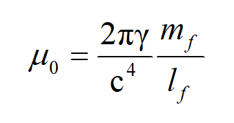
describing the Magnetic Constant
using only the FUNDAMENTAL MEASURES
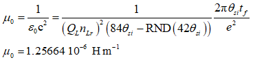
2018 CODATA Measure
1.25664 10-6 H m-1
MQ Calculation
1.25665 10-6 H m-1
Inputs
- θsi can be measured as the polarization angle of quantum entangled X-rays at the degenerate frequency of a maximal Bell state. As an angle θsi=3.26239 rad ± 2 μrad; as a momentum θsi=3.26239030392(48) kg m s-1 and with respect to the Target Frame, θsi has no units. The relation of angle and mass is mathematically demonstrated, as well, by No-Ping Chen, et. al.
- lf, mf and tf are the fundamental measures, more precise expressions for Planck’s units – length, mass, and time – that consider the effects of length contraction associated with discrete measure.
Terms
- c is the speed of light which may also be written as c=nLlf/nTtf=299,792,458 m/s such that nL=nT=1 is physically significant.
- QL is the fractional portion of a count of lf when engaging in a more precise calculation.
- nLr describes the count of lf representative of the position of an observable with respect to the frame of a center of mass.
- Δf is the metric differential; describes the numerical difference in distance between the discrete and non-discrete frames of reference.
- QLnLr, also known as the Informativity differential describes the length contraction associated with discrete measure.
- ɛ0 is the electric constant
- μ0 is the magnetic constant
- e is elementary charge
- ħ is the reduced Planck constant, 1.054571817 10-34 m2 kg s-1. When accounting for the Informativity differential at the upper count bound, this term is not italicized (i.e., ħ=1.0545349844(45) -34 m2 kg s-1).
- αf-1 is the fundamental form of the inverse fine structure constant defined with respect to the Target Frame.
- αp-1 is the Planck-like form of the inverse fine structure constant defined with respect to the Measurement Frame.
- αc-1 is the classical form of the inverse fine structure constant as adopted by the CODATA collaboration. This term accounts for length contraction associated with discrete measure.
- γ is a collection of terms that describe the geometry between the Target and Measurement Frames.
Calculations

Experimental Support

NIST: CODATA Recommended Values of the Fundamental Physical Constants: 2018, (May 2019), https://physics.nist.gov/cuu/pdf/wall_2018.pdf, doi:10.1103/RevModPhys.93.025010.
Discussion
Given the correlation between the electric and magnetic constant μ0=1/ɛ0c2, one might conclude that neither is more fundamental than the other. Yet, when presenting these expressions using an MQ nomenclature we do not find this to be the case. Looking to expressions such as the correlation between G and ɛ0 or the correlation between α and ɛ0, we find the magnetic constant to be a physical extension of the two in magnitude by c2. It is as such that we begin with a review of expressions presented in the paper entitled, Describing the Electric Constant ....
First, we offer a technical note regarding a change in how physical constants are resolved. With the May 2019 redefinition of the electric and magnetic constants, the magnetic constant is now a measured value with the electric constant calculated. Considering definitions offered by MQ, both can be calculated as a function of the fundamental measures alone. That said, we adhere to convention using the magnetic constant as a source measure for the fundamental measures, when describing other constants such as the fine structure constant and the reduced Planck constant.
We proceed by first resolving the difference between frames, the non-discrete System Frame and the discrete Internal Frame of the universe.

We must also account for the length contraction effects described by the Informativity differential. In this case, we are concerned with the length associated with the measure of blackbody demarcation. Notably, the effect increases in magnitude with decreasing distance.

And with these results we can present three expressions describing the fine structure constant. The first we call the fundamental form of the inverse fine structure constant. In this form, the expression is defined with respect to the System Frame of the universe. After applying the metric differential between frames we resolve its Internal Frame definition, what we call its Planck-like form. Planck's expressions are by default in this form, in that they do not account for the length contraction effects associated with a discrete internal frame. Finally, accounting for this effect - the Informativity differential - we resolve its classical form, what is measured in the laboratory. This expression corresponds with the today's existing classical expressions with one notable difference. We resolve the physical constants using only the fundamental measures, a physically distinct measurement framework. Resolved values match existing measures digit for digit.

With solutions for each of the components, we can then resolve a general expression for the electric constant.

And using μ0=1/ɛ0c2 and c=lf/tf, we resolve the magnetic constant.
But we still must resolve an MQ expression for elementary charge. A metric description of elementary charge is lengthy with several physical considerations that must be accounted for. Once completed, the final expression is then

And finally, we replace e in our expression for the magnetic constant (above) to resolve a MQ description of the magnetic constant.
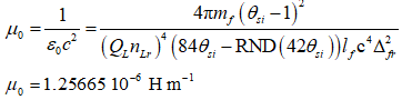
Comparing the results to the 2018 CODATA, we find a difference of one part in the sixth digit. In the table below, we extend the precision of this calculation using an approach to resolving elementary charge, called the gamma approach. This is to say, ec is a physically significant approach to its calculation. More research is needed to improve accuracy, but in the meantime we are able to resolve the value of gamma as a function of unrelated measures - a calculated value - and then use that to resolve MQ expressions for the electromagnetic constants. This provides us with digit-for-digit correspondence equal to our best measurements.
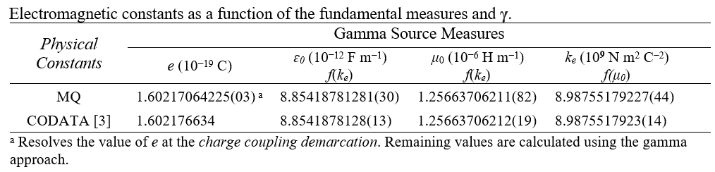
NIST: CODATA Recommended Values of the Fundamental Physical Constants: 2018, (May 2019), https://physics.nist.gov/cuu/pdf/wall_2018.pdf, doi:10.1103/RevModPhys.93.025010.
Notably, the calculations represent a small sampling of concepts. One, there is a frame difference which must be accounted for between the discrete and non-discrete frames. Then there is a skewing in the measure of length lf, a function of the distance associated with the blackbody demarcation. There is also a geometry related to elementary charge which we present as a function of θsi. And finally, there is π, a physically significant value correlating particle and wave phenomena, in this case those descriptions correlate classical motion with electromagnetic phenomena. Collectively, these are the principles that underlie a description of magnetism and relate that description with all other phenomena.

Quantum Inflation, Transition to Expansion, CMB Power Spectrum