—————————— read pre-print on research gate (new window) ——————————

• θ_si, is 3.26239 radians or kg m/s (momentum) or no units at all a function of the chosen frame of reference. This is a new constant to modern theory and exists in nearly every equation of the model. It may be measured macroscopically given specific Bell states necessary for quantum entanglement of X-rays such as those carried out by Shwartz and Harris.

• r_q is a term representing a quantization ratio. The value of a ratio is not directly correlated with a particular phenomenon, but indirectly describes the mathematical correlation between the discrete and non-discrete frames of reference.
• n is any number multipled by θ_si. The value of n does not need to be integer as is usually the case with counts. Although whole-unit values of n are physically significant, decimal values can be used to resolve physically significant constants in nature.

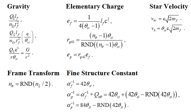
We offer calculations of the fine structure constant as one example where a quantization ratio is used. The fine structure constant uses the most basic form of r_q to resolve the count difference between l_f in the Measurement Frame and θ_si in the Target Frame (i.e., RND(84.6/2)=42, thus α_f⁻¹=42θ_si). Note, the value 84.6 is the count nLr associated with blackbody radiation.

With this, we then use the difference between the discrete and non-discrete products of this pair to resolve the metric differential associated with this measure. This also provides us with the Planck-like form of the expression α_p⁻¹. Finally, we account for the length contraction associated with discrete measure - also called the Informativity differential. This gives us the classical form of the expression α_c⁻¹, what is compared with measurements made under ordinary laboratory conditions. We identify the calculation associated with this measure as the charge coupling demarcation. Notably, there is no difference.

The term quantization ratio r_q describes the relation of the non-discrete Target Frame of the universe to the discrete Measurement Frame of the observer with regards to the measure of a phenomenon. There are three classes of expressions used to resolve this relation.

The first regards the count of l_f as observed in the Measurement Frame relative to the count of θ_si as calculated in the Target Frame. This ratio is solidly known as a division by two, thus resolving the Target Frame count.

The second frame transform is described by a difference. An example of its implementation is used in the presentation of expressions for the fine structure constant. Specifically, using the first transform to resolve the base count of 42θ_si relative to the Target Frame, we resolve its Measurement Frame description as the difference between the discrete and non-discrete product of these two values.

The third frame transform is described by a ratio. We call this a quantization ratio. An example of its use is provided in the presentation of expressions for elementary charge. A verbal description would be difficult, but we can summarize in general that charge is resolved as a discrete offset of the equality of the second and third transforms, resolved at the lower count bound to fundamental measures. We add that we can demonstrate the solution is physically significant, but we admit it is also incomplete. Thus, precision is limited to six digits, as opposed to any other Measurement Quantization (MQ) calculation which demonstrates up to 13 digits of digit-for-digit correspondence, this being the most precise measurements available at this time.

To provide additional detail as to how these calculations are carried out we will continue with a more detailed explanation of frames of reference. MQ involves use of a novel nomenclature of counts n_L, n_M, and/or n_T of fundamental units of measure l_f, m_f, and/or t_f to account for three properties of measure. Those properties can be mathematically resolved relative to the Reference, Measuement and Target frames with an analysis of Heisenberg’s uncertainty principle, the speed of light and the expression for escape velocity. The properties of measure are, discreteness, countability and in reference to three frames of reference. We define the three frames such that there is a:

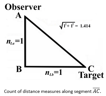
• Reference Framework — This is the framework of the observer where properties of the reference (AB) are observed. With respect to the standard understanding, this framework differs only in that measure is a count function of discrete length measures equal to one.
• Measurement Framework — This framework shares properties with the Reference Framework. It is characterized as some known count of the reference describing where count properties of the reference (BC) are observed.
• Target Framework — This framework is characterized by the property of measure of non-discreteness, that being the framework of the universe that contains the phenomenon (AC).

Quantization ratios offer a physically significant approach to resolving expressions and values for the physical constants. They describe the geometry between the non-discrete and discrete frames. Thus, if a count of θ_si is known in the non-discrete frame, quantization ratios can be used to resolve its corresponding value in the discrete frame.

For instance, quantization ratios can be used to understand the ground state orbital of an atom. They can also be used to resolve the value of Planck’s constant. And where used in combination with other frame transforms, we can resolve the metric differential associated with several constants and phenomena, as displayed in the table below. Therein, we grasp a deeper understanding of the construct of our universe.