—————————— read pre-print on research gate (new window) ——————————

• θ_si can be measured as the polarization angle of quantum entangled X-rays at the degenerate frequency of a maximal Bell state. As an angle θ_si=3.26239 rad ± 2 μrad; as a momentum θ_si=3.26239030392(48) kg m s^-1 and with respect to the Target Frame, θ_si has no units. The relation of angle and mass is mathematically demonstrated, as well, by No-Ping Chen, et. al.

• Q_L is the fractional portion of a count of l_f when engaging in a more precise calculation.
• Q_Ln_Lr, also known as the Informativity differential describes the length contraction associated with discrete measure.
• n_Lr describes the count of l_f representative of a change in position of an observable measured with respect to the observer’s frame of reference.
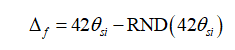
• Δ_f is the metric differential between frames associated with the fine structure constant.
• α_f^-1 is the fundamental form of the inverse fine structure constant defined with respect to the Target Frame.
• α_p^-1 is the Planck-like form of the inverse fine structure constant defined with respect to the Measurement Frame.
• α_c^-1 is the classical form of the inverse fine structure constant as adopted by the CODATA collaboration. This term accounts for length contraction associated with discrete measure.

The fine structure constant α describes the strength of the coupling of an elementary charged particle with the electromagnetic field. Named by Arnold Sommerfeld in 1916, he used α as a physical constant to extend the Bohr model, describing gaps in the spectral lines of hydrogen atoms.

Using Measurement Quantization (MQ) we extend our understanding of α. Whereas Sommerfeld approached this value from the point-of-view of the Bohr atom^{(6,Eq. 64)}, whereas Planck incorporated this value into an expression describing the ground state orbital of an atom^{(6,Eq. 63)}, we present a foundation that correlates both descriptions and a third (a fundamental description^{(6,Eq. 62)}) into a single physically correlated presentation. Incidentally, the inverse fundamental fine structure constant is 42θ_si, such that θ_si is the radial rate of universal expansion. θ_si is also the Planck momentum and can be measured as the polarization angle of quantum entangled X-Rays at their degenerate frequency, specifically at the maximum in angle.

With this base description, we account for for frames of reference and a length contraction effect associated with discrete measure. The term α_f differs from the Planck expression by the difference between frames. There are three^{(6,Sec. II.D)}; the Reference, the Measurement, and the Target Frame. The first two are discrete corresponding to the self-referencing framework of the observer. The Target Frame describes the self-defining non-discrete framework of the universe. Why is the universe non-discrete? Because it has no external frame with which to provide reference. In that the universe expands at the speed-of-light, it is not possible for the universe to have an external frame of reference.

The difference between the two frames we call the metric differential.

Next we account for length contraction. We call this effect the Informativity differential Q_Ln_Lr. It describes the skew in measure associated with discrete measure. The effect is a distance sensitive property, largest at quantum distances. Notably, the expression can also be used to resolve the count n_Lr associated with a phenomenon. We identify this count as a demarcation. For instance, the count associated with blackbody radiation we call the blackbody demarcation.

With these evaluations, we can now correlate the three descriptions to resolve what is measured in the laboratory. We begin with the inverse fundamental fine structure constant^{([6], Eqs. 62-64)}. We then add the metric differential to resolve the inverse Planck-like fine structure constant. And finally, we subtract two times the Informativity differential to resolve the classical form of the inverse fine structure constant.

As displayed in the table below, all values match to twelve significant digits. We have included a difference column which describes the difference between the MQ calculation and the CODATA measures to 13 significant digits. You will note that the values are the same, revealing a physical correlation between each calculation and its measured value within the bounds of the corresponding measurement precision.

These calculations serve as a foundation to unraveling much of electromagnetic theory and correlating this discipline to the other fields … notably, their unification with the phenomenon of gravitation^{(6,Sec. III.D)}. At a higher level, we find once again that all values may be understand entirely as a function of θ_si.