

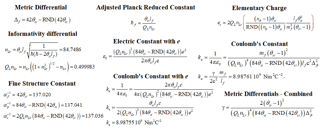
describing Coulomb’s Constant
using only THE FUNDAMENTAL MEASURES
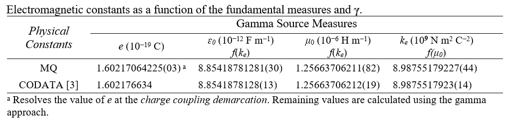
2018 CODATA
MQ
8.9875517923(14) 109 N m2 C-2
8.98755179227(44) 109 N m2 C-2
Inputs
- θsi, is 3.26239 radians or kg m/s (momentum) or no units at all a function of the chosen frame of reference. This is a new constant to modern theory and exists in nearly every equation of the model. It may be measured macroscopically given specific Bell states necessary for quantum entanglement of X-rays such as those carried out by Shwartz and Harris.
- lf, mf and tf are effectively Planck’s Units for length, mass and time, but not precisely the same. In MQ we recognize them as the fundamental units.
Terms
- c is the speed of light which may also be written as c=nLlf/nTtf=299,792,458 m/s such that nL=nT=1 is physically significant.
- QL is the fractional portion of a count of lf when engaging in a more precise calculation.
- nLr describes the count of lf representative of the position of an observable with respect to the frame of a center of mass.
- Δf is the metric differential; describes the numerical difference in distance between the discrete and non-discrete frames of reference.
- QLnLr, also known as the Informativity differential describes the length contraction associated with discrete measure.
- ɛ0 is the electric constant
- μ0 is the magnetic constant
- e is elementary charge
- ħ is the reduced Planck constant, 1.054571817 10-34 m2 kg s-1. When accounting for the Informativity differential at the upper count bound, this term is not italicized (i.e., ħ=1.0545349844(45) -34 m2 kg s-1).
- αf-1 is the fundamental form of the inverse fine structure constant defined with respect to the Target Frame.
- αp-1 is the Planck-like form of the inverse fine structure constant defined with respect to the Measurement Frame.
- αc-1 is the classical form of the inverse fine structure constant as adopted by the CODATA collaboration. This term accounts for length contraction associated with discrete measure.
- γ is a collection of terms that describe the geometry between the Target and Measurement Frames.
- ke is Coulomb’s constant.
Calculations
Experimental Support
[3] NIST: CODATA Recommended Values of the Fundamental Physical Constants: 2018, (May 2019), https://physics.nist.gov/cuu/pdf/wall_2018.pdf, doi:10.1103/RevModPhys.93.025010.
Discussion
We find Coulomb’s constant to be an extension of the electric constant. In comparison to the inverse of the electric constant we take its product with the matter/wave correlation – cancelling out this dimension – to resolve Coulomb’s constant. The effect is like taking length divided by time and multiplying by mass to go from a description of the speed-of-light to a description of the Planck momentum. In the same way, each example identifies a bound to measure with respect to an arrangement of dimensions.
On the other hand, the value of Coulomb’s constant as a physically significant descriptor along with its component descriptors is more a matter of convenience than physical significance. We will move through the calculation quickly, referring the reader to those articles on frames of reference, the Informativity differential, the fine structure constant and the electric constant to untangle the greater significance of those component terms that make up Coulomb’s constant. We will also forego the typical lengthy explanation of how these classical concepts are defined, based on the understanding that the content in supporting articles is accessible if needed.
Thus, where there are three physically significant frames of reference – the Reference, Internal and System Frames – we take the difference between the Internal and System frames to resolve the metric differential.

We will also need to account for the length contraction associated with the discrete measure relative to the Internal Frame, described by the Informativity differential. The effect is a property of measures having two or more dimensions, as described in several published papers [1-6]. While this count difference is an outcome of the Pythagorean theorem, the count nL of lf associated with blackbody radiation must be resolved in advance. We recognize this count as the blackbody demarcation.

With these two measures and associated calculations, we can resolve an expression for the inverse fine structure constant. We begin, as noted earlier, with its fundamental form and then apply the metric differential followed by the Informativity differential to resolve an expression and value for what we call its classical form, also described in macroscopic form using mostly electromagnetic terms as published with any publication of the CODATA.

A partially resolved form of the electric constant can then be resolved with these expressions.

And this can be applied to a description of Coulomb’s constant.

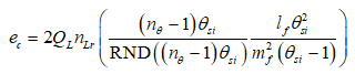
And finally, we require a discrete description of elementary charge. Elementary charge is a very difficult phenomenon as there appears to be no known solution as a function of θsi defined with respect to the non-discrete System frame. As such, we use our understanding of the relation between the Internal and System frames to resolve a description in terms of the fundamental measures. This is written as,
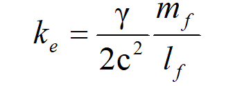
And then replacing e, we resolve Coulomb’s constant as a function of θsi and the fundamental measures. We also replace both the metric and Informativity differential with gamma γ.
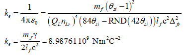
We can then compare the results with their corresponding 2018 CODATA published values.

[3] NIST: CODATA Recommended Values of the Fundamental Physical Constants: 2018, (May 2019), https://physics.nist.gov/cuu/pdf/wall_2018.pdf, doi:10.1103/RevModPhys.93.025010.

Quantum Inflation, Transition to Expansion, CMB Power Spectrum