—————————— read pre-print on research gate (new window) ——————————

• θ_si can be measured as the polarization angle of quantum entangled X-rays at the degenerate frequency of a maximal Bell state. As an angle θ_si=3.26239 rad ± 2 μrad; as a momentum θ_si=3.26239030392(48) kg m s^-1 and with respect to the Target Frame, θ_si has no units. The relation of angle and mass is mathematically demonstrated, as well, by No-Ping Chen, et. al.
• l_f, m_f and t_f are the fundamental measures, more precise expressions for Planck’s units – length, mass, and time – that consider the effects of length contraction associated with discrete measure.

• Q_Ln_Lr, also known as the Informativity differential describes the length contraction associated with discrete measure.
• Q_L is the fractional portion of a count of l_f when engaging in a more precise calculation.
• n_Lr describes the count of l_f representative of the position of an observable with respect to the frame of a center of mass.
• h is Planck’s constant.
• ħ is the reduced Planck constant, 1.054571817 10^-34 m² kg s^-1. When accounting for the Informativity differential at the upper count bound, this term is not italicized (i.e., ħ=1.0545349844(45) ^-34 m² kg s^-1).
• r_q is the quantization ratio (n_θθ_si)/RND(n_θθ_si). It describes the relation between the discrete and non-discrete frames of reference.
• RND(n) is a function; round to the nearest whole-unit value.

In addition to the well-known classical expressions for the reduced Planck constant, MQ offers an alternative. We approach the calculation anew, as a function of the Planck momentum θ_si which in turn is resolved as a measure of the fine structure constant. Several principles are needed to carry out the calculation.

The first regards frames of reference. There are three physically significant frames needed to describe any phenomenon. They are, the:

• Reference Framework — This is the framework of the observer where properties of the reference (AB) are observed. With respect to the standard understanding, this framework differs only in that measure is a count function of discrete length measures equal to one.
• Measurement Framework — This framework shares properties with the Reference Framework. It is characterized as some known count of the reference describing where count properties of the reference (BC) are observed.
• Target Framework — This framework is characterized by the property of measure of non-discreteness, that being the framework of the universe that contains the phenomenon (AC).

Of these, there are also two significant domains of physical description. The first domain includes the description of phenomena with respect to other phenomena in the universe. The second domain includes the description of phenomena with respect to the universe.

We identify first domain descriptions as the self-referencing Measurement Frame of the observer; that is, descriptions that are a function of the internal reference measures for length, mass, and time. Conversely, the universe has no external reference. We refer to such descriptions as being a function of the self-defining Target Frame of the universe. Importantly, it follows that Target Frame descriptions are non-discrete, there being no external reference frame work. The internal system is discrete.

In addition to frames the reader will also need to be familiar with quantization ratios. Quantization ratios present a mathematical approach that allows us to correlate descriptions of phenomenon with respect to the discrete and non-discrete frames. The expression for a quantization ratio is

The count term n, in this case, can take on any iteger value. [Quantization ratios][2] provide a discreete mathematical approach to correlating the Target and Measurement Frames relative to the measurment bound. For instance, with respect to a description of elementary charge, its discrete description can be resolved by setting the bound quantization ratio (a fractional relation) equal to the difference. Another way to describe this is b-d=b/d at the lower measurement bound.

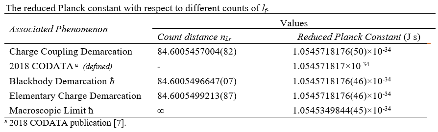
Length contraction as found associated with discrete measure must also be accounted for. This effect can be used to resolve a demarcation distance associated with each phenomenon. Thus far, we have resolved demarcations associated with blackbody demarcation, elementary charge and charge couplings, n_Lr=84.60055. The values differ in the seventh digit, but otherwise can be used interchangeably to resolve the value of their associated phenomenon to 14 significant digits.

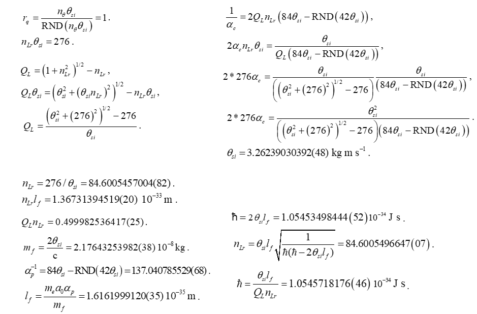
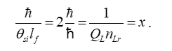
With these principles we can approach a calculation of the reduced Planck constant by resolving the demarcation associated with blackbody radiation Q_Ln_Lr, the Planck momentum θ_si and fundamental length l_f. Thus,

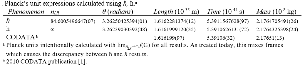
When compared to the 2018 CODATA we find the value for ħ matches to ten digits, the same digit-for-digit correspondence as its existing defined value.

We bring to the reader's attention that the first solution is resolved with respect to the upper count bound. As such, we do not italicize the symbol. The latter is resolved with respect to the demarcation. We have resolved the demarcation as a function of the defined value, but do not use this value to then resolve the value for ħ at the demarcation. Rather, the last calculation is carried out with respect to the elementary charge demarcation, as a representative proxy for this phenomenon. Otherwise, we'd simply resolve in calculation the initial defined input for ħ.

Finally, we consider a graphical presentation of ħ as a function of the Informativity differential. Setting x=ħ_f/θ_sil_f and y=1/n_Lr., we then have

The function may then be graphed to describe the magnitude of the Informativity differential^{(6,Sec. II.G)} relative to the distance of an observed object. More importantly, we find that the vertex of the right parabola marks the count distance n_θ that corresponds to the blackbody demarcation^{(6,Apx. C)}.

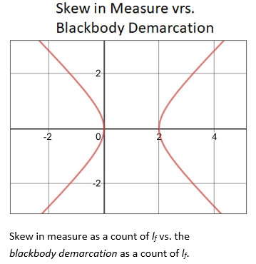
The solution as displayed in the graph above for ħ/θ_sil_f falls on the point (2.000069857, 0.000139718) on the right parabola. The axis of symmetry for both parabolas lie parallel to the x-axis. The expression can also be reduced. With ħ_f=2θ_sil_f and ħ=θ_sil_f/Q_Ln_Lr, then

Substituting 1/Q_Ln_Lr for ħ/θ_sil_f, then

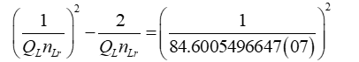
Written as such we find that the graph is a representation of a plane with both axis describing counts of l_f. Importantly, while the physical significance of the blackbody demarcation is somewhat understood, what is the physical significance of the vertex on the left parabola, with x and y coordinates that are each positive. Is this a physically important quality of the vacuum of space?

At present, we theorize that mass accretion in the universe is not entirely random, but instead a fixed rate function such that particles accrete near existing mass. This is to say that not all spacetime is equally conducive to the retention of new mass accreting into the universe. And as such, particles that do accrete into the universe are most likely to occur near existing mass. This can be modeled and validate with respect JWST observations regarding proto-galaxy formation. A peer-reviewed paper regarding this effect is the subject of a future paper.