

describing the Electric Constant
using only the FUNDAMENTAL MEASURES

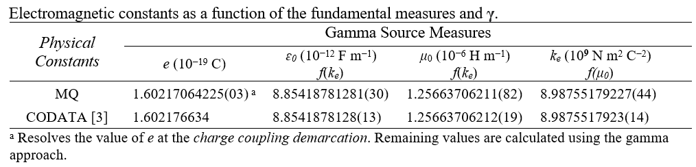
2018 CODATA
MQ
8.8541878128(13) 10-12 F m-1
8.85418781281(30) 10-12 F m-1
Inputs
- θsi can be measured as the polarization angle of quantum entangled X-rays at the degenerate frequency of a maximal Bell state. As an angle θsi=3.26239 rad ± 2 μrad; as a momentum θsi=3.26239030392(48) kg m s-1 and with respect to the Target Frame, θsi has no units. The relation of angle and mass is mathematically demonstrated, as well, by No-Ping Chen, et. al.
- lf, mf and tf are the fundamental measures, more precise expressions for Planck’s units – length, mass, and time – that consider the effects of length contraction associated with discrete measure.
Terms
- c is the speed of light which may also be written as c=nLlf/nTtf=299,792,458 m/s such that nL=nT=1 is physically significant.
- QL is the fractional portion of a count of lf when engaging in a more precise calculation.
- nLr describes the count of lf representative of the position of an observable with respect to the frame of a center of mass.
- Δf is the metric differential; describes the numerical difference in distance between the discrete and non-discrete frames of reference.
- QLnLr, also known as the Informativity differential describes the length contraction associated with discrete measure.
- ɛ0 is the electric constant
- μ0 is the magnetic constant
- e is elementary charge
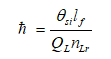
- ħ is the reduced Planck constant, 1.054571817 10-34 m2 kg s-1. When accounting for the Informativity differential at the upper count bound, this term is not italicized (i.e., ħ=1.0545349844(45) -34 m2 kg s-1).
- αf-1 is the fundamental form of the inverse fine structure constant defined with respect to the Target Frame.
- αp-1 is the Planck-like form of the inverse fine structure constant defined with respect to the Measurement Frame.
- αc-1 is the classical form of the inverse fine structure constant as adopted by the CODATA collaboration. This term accounts for length contraction associated with discrete measure.
- γ is a collection of terms that describe the geometry between the Target and Measurement Frames.
Calculations

Experimental Support

[3] NIST: CODATA Recommended Values of the Fundamental Physical Constants: 2018, (May 2019), https://physics.nist.gov/cuu/pdf/wall_2018.pdf, doi:10.1103/RevModPhys.93.025010.
Discussion
The electromagnetic constants are best described as internal frame descriptions in part a function of the fine structure constant, elementary charge and Planck’s constant. The remaining terms sometimes appear singularly or as a function of one another: the electric constant, the magnetic constant and Coulomb’s constant. With respect to a Measurement Quantization (MQ) approach, this is consistent with expressions described wholly within the Internal Frame. Breaking the deadlock is difficult without a firm understanding of frames of reference and how the forces of nature are related. Many have suspected that a quantum - as in quantum mechanical - description of gravity would allow for a breakthrough. This has not been the case. We present a new approach with which to resolve the electric constant, now in terms of the fundamental measures.
Notably, we call to the reader's attention that most if not each of the descriptions we present are counts of the fundamental measures and/or the fundamental measures. We do not use the physical constants as component terms to a final definition of the electromagnetic constants. We do introduce two geometries.
Those geometries describe the relation of the Internal and System frames. The first, the metric differential, describes the relation of θsi between the System frame of the universe and its Internal frame. For brevity, if you are not familiar with frames of reference and their physical significance, please see the respectively linked articles.

The second effect we call the Informativity differential. It describes the skew in measure associated with discrete measure (i.e. 2QLnLr). The effect is a distance sensitive property of measure that decreases in magnitude with increasing distance. Unlike the contraction of length described by relativity, this effect is unrelated, a geometric consequence best understood when approached using the Pythagorean theorem.

Understanding these effects is important to resolving, for instance, the fundamental form of the fine structure constant (6,Eq. 62). A fundamental description is resolved against the System Frame. Taking into account the metric differential between frames, we resolve the Planck-like form of the same expression. And finally, accounting for the Informativity differential, we resolve the classical form of the expression, its electromagnetic equivalent as would be found in the most recent publication of the CODATA.
We bring to the reader's attention, historically speaking, there exists no explanation for the calculated difference between the Planck and electromagnetic expressions for the fine structure constant or for that matter any Planck description and its corresponding electromagnetic description. This we resolve as a physically significant consequence of the Informativity differential. A mathematical implementation describing the inverse fine structure constant is:

Next, we also need a description of the reduced Planck constant, one that incorporates the length contraction effects described by the Informativity differential. To distinguish how a measure is resolved, we modify the nomenclature. Terms are not italicized when their measure is taken at the upper count bound. All other measures - for instance, the measure of ħ with respect to blackbody radiation - are written in italics.
With MQ descriptions of each component term, we can resolve the electric constant ɛ0. The expression is not entirely reduced in that there does not exist a fundamental expression for elementary charge. We will use e initially and then return to consider the gamma approach, which isolates an approximation and then encapsulates that inside a new term - gamma - which can be resolved separately with 13 digits of physical significance.

In the next expression, we resolve elementary charge as a function of θsi in terms of the fundamental measures(5,Sec. III.B). The presentation involves several steps which are discussed in the respective article. For our purposes, we present the solution.

And with this we then replace elementary charge. This allows us to resolve the electric constant as a function of θsi and the fundamental measures.

Compared to the most recent CODATA, there is a difference in the sixth digit. Notably, the measure of θsi is constrained to six digits of precision when using the Shwartz and Harris model and measurements as a source. As such, some variation in the sixth digit is expected.
[3] NIST: CODATA Recommended Values of the Fundamental Physical Constants: 2018, (May 2019), https://physics.nist.gov/cuu/pdf/wall_2018.pdf, doi:10.1103/RevModPhys.93.025010.
To extend precision, we use the gamma approach to resolve a value for gamma and with respect to the electric, magnetic constants and the Coulomb. Notably, all solutions to gamma are the same to eleven digits. It follows if precision equal or less are all that are desired, then it is irrelevant which source measure is resolved. Otherwise, we select a source physically independent of the calculation we seek to resolve. In this case, we present the electric constant as a function of the Coulomb. The resultant calculation for the electric constant shows no difference with the CODATA.

Quantum Inflation, Transition to Expansion, CMB Power Spectrum