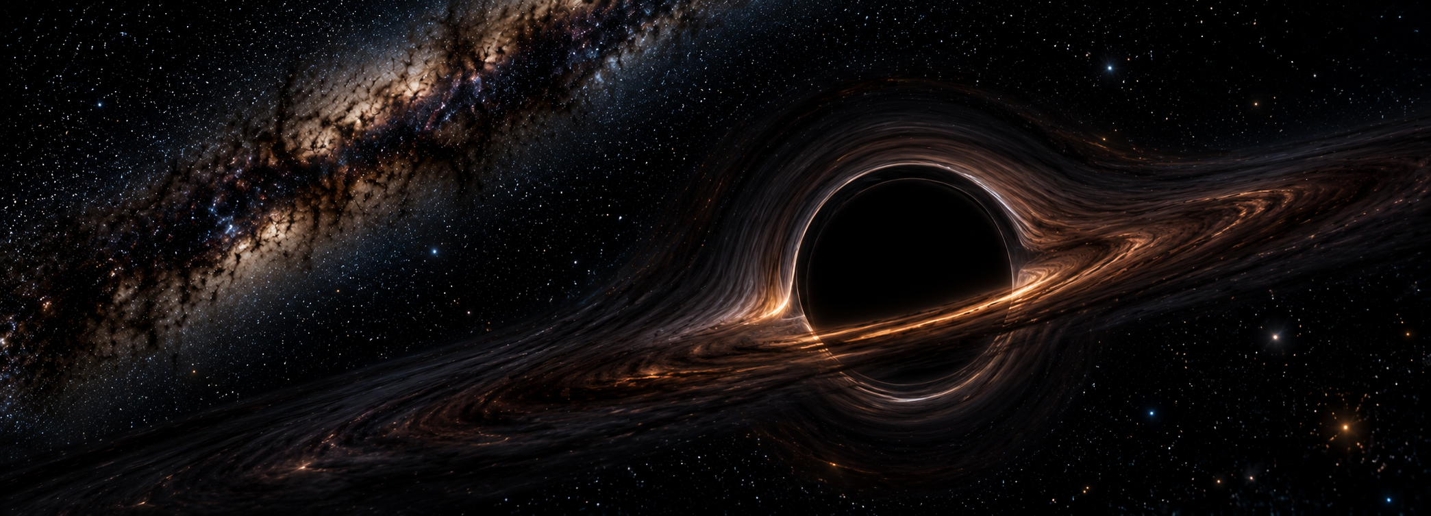
Singularity Exclusion in the Bounded Measurement Quantization Domain

Jody A. Geiger

Informativity Institute

Chicago, IL USA 60605

jodygeiger@informativity.org

ORCID: 0000-0001-5389-0447

ABSTRACT

Measurement Quantization (MQ) describes physical measure through reference counts and their observer–observable realization. The Internal Frame is the discrete configuration domain; the System Frame is its continuous relational encoding induced by the Frames mapping. The bounded MQ admissibility domain requires that positive whole-unit measures in the measurement domain have counts no smaller than one and a finite upper count set by the normalized reciprocal of fundamental time. Local measures belong to the framework of the observable, whereas observed measures belong to the framework of the observer. Their count relations give common length and time factors and reciprocal observed-mass dilation. The speed substitution reproduces the Lorentz square-root factor. Applying the minimum count to the observed measure as well as the local reference excludes a zero transformation factor. With the finite upper count, the admissible factors remain separated from zero and physical measures remain finite. Thus zero or infinite measure is excluded within this bounded MQ domain. Numerical calibration uses the 2022 adjustment of the Committee on Data of the International Science Council (CODATA).

Keywords: Singularities, Physical Significance, Measure, Discrete

1. INTRODUCTION

Using a physically correlated description of measure, we examine how MQ excludes singularities from its admitted physical measurement domain. Here a singularity means a physical description in which a positive measure tends to zero or grows without a finite bound. The claim concerns the positive measures represented by MQ, rather than every divergence that can be written in a continuous mathematical extension. The speed of light, escape velocity and Heisenberg’s uncertainty principle [1] motivate the reference construction in [2]. Counts belong to the Internal Frame configuration domain, while dimensions and observable relations arise in the System Frame through the Frames mapping.

The realized fundamental measures are l_f, m_f and t_f, with units m, kg and s. They are distinguished from conventional Planck units [3]. Their dimensionless counts n_L, n_M and n_T refer here to radial separation, source mass and elapsed time. The distinct motion count n_Lm records the change in realized position of an observed mass. Internal count expressions are representational; their corresponding dimensioned quantities are obtained through the Frames mapping. The finite upper count used below restricts the admitted configuration in the stated measurement domain, rather than an accumulated total over successive configurations.

We compare count descriptions with the relativistic setting [4, 5]. Let M=n_Mm_f be source mass in kg and r=n_Ll_f radial separation in m. The speeds v and c have units m s⁻¹, with v the common motion parameter and c the speed of light. The dimensionless light-travel count n_Lc uses the same elapsed-time count as n_Lm, giving v=n_Lml_f/(n_Tt_f) and c=n_Lcl_f/(n_Tt_f). The ratio is therefore v/c=n_Lm/n_Lc. The classical escape speed v_e is used to establish

v_{e}^{2} / c^{2} = 2 n_{M} / n_{L}

([2], Appx. AV, Eqs. (AV.2)–(AV.4)). The strict exterior condition is n_M/n_L<1/2 ([2], Appx. O). Its identification with the motion ratio is stated explicitly in Eq. (12).

The exclusion argument uses the MQ reference counts and the observation relations already introduced. It requires no additional particle, force or extra dimension within that construction. Inflation [6], loop quantum gravity [7, 8] and string theory [9] are distinct research programs; they are not evaluated by the present count-bound argument. The numerical realization is calibrated to the stated 2022 input, so its precision does not constitute an independent test of MQ.

The historical count and framework discussion in [2], Appx. I–K, supplies background for the current interpretation used here. Discrete count configurations belong to the Internal Frame, whereas the System Frame continuously encodes their relational realization through the Frames mapping. The bounded-measure argument uses this distinction without asserting that it determines whether the universe, considered without a specified measurement framework, is discrete or continuous.

Within this framework distinction, a local measure of the observable and the measure assigned by an observer are distinct quantities. Their reference frameworks determine the contraction and dilation factors examined below. The separation of configuration and realization also underlies the MQ calculations of physical constants in [10].

2. METHODS

This paper integrates the count relations with their physical admissibility conditions. We identify the approach as Measurement Quantization (MQ), with applications discussed in [2, 10, 11, 12, 13, 14, 15]. Positive observed counts must obey the same stated count-domain restrictions as their local references. The finite bound and the observed/local comparison are separate premises; the exclusion of singular measures follows by applying them together.

Measurement Quantization [2] develops the reference construction and discusses comparisons with physical measurements. We use that construction as the mathematical basis of this paper. Those comparisons motivate the MQ description; they do not independently establish the finite-count exclusion proved here. The numerical inputs and their propagated uncertainties are stated in Appendix A.

https://www.researchgate.net/publication/361148724_OnlineResources

The supplementary spreadsheets described in [2] provide calculations for the introductory construction and its applications. The present argument is specified by the equations, admissibility conditions and numerical calibration given below. Its conclusion does not depend on an asserted verification of every supplementary calculation or of all the related applications.

3. RESULTS

The singular descriptions defined in Sec. 1 arise when a mathematical expression is extended toward zero or unbounded physical measure. The question here is whether that continuation remains within the admitted MQ count domain. We first bound ordinary ratios and then examine the square-root and reciprocal factors.

MQ reduces the measures considered here to fundamental references and their counts. The invariant coefficient θ_si is dimensionless and enters their calibration. The six ratios n_M/n_L, n_M/n_T, n_L/n_M, n_L/n_T, n_T/n_L and n_T/n_M are dimensionless. If both counts of a ratio obey the positive finite domain below, the ratio cannot vanish or become infinite. The transformation expressions require a further check because a difference of count ratios could otherwise make a square-root factor zero. We therefore apply the minimum observable count to the transformed measure.

The MQ lower bound adopted here is one for every positive whole-unit count admitted in this observer–observable measurement domain (compare the discreteness discussion in [2], Appx. J). Zero denotes absence of the corresponding measure. The primitive boundary construction n_L=n_T=1, n_M=1/2 is retained in Eq. (14) to identify the zero-factor boundary; it is not an admitted positive whole-unit observer configuration. The physical domain for the transformations also requires the observed measures to have positive admissible counts.

The reciprocal fundamental time 1/t_f is a rate in s⁻¹ ([2], Appx. O). Equations (1)–(3) calculate the common reference rate for a one-second normalization using 2022 CODATA inputs [16]. Multiplication by the exact normalization interval converts it into the dimensionless upper-bound parameter n_max adopted for this domain. Equation (1) uses the light-travel count; the mass and time counts in Eqs. (2) and (3) are evaluated at their corresponding reference-rate benchmarks, rather than as a simultaneous admitted source configuration. This upper bound belongs to the MQ admissibility domain; the reference-rate conversion fixes its normalized numerical scale. In Eq. (4), n is a manuscript-local placeholder for any admitted positive whole-unit reference count; it introduces no additional MQ primitive. Parentheses give one standard uncertainty in the final digits. The reported upper-bound parameter is not a determination of a unique endpoint integer.

\frac{n_{Lc}}{1 ​ s} = \frac{c}{l_{f}} = 1.85492188108 (14) \times 10^{43} ​ s^{- 1}

(1)

\frac{n_{M}}{1 ​ s} = \frac{4.03711234219 (62) \times 10^{35} ​ kg ​ s^{- 1}}{m_{f}} = 1.85492188108 (14) \times 10^{43} ​ s^{- 1}

(2)

\frac{n_{T}}{1 ​ s} = \frac{1}{t_{f}} = 1.85492188108 (14) \times 10^{43} ​ s^{- 1}

(3)

n_{\max} = \frac{1 ​ s}{t_{f}} = 1.85492188108 (14) \times 10^{43}, ​ 1 \leq n \leq n_{\max}

(4)

Equation (4) applies the finite bound to source, local and observed counts in the admitted domain. A ratio of any two such positive counts lies between 1/n_max and n_max, so ordinary count ratios have neither a zero limit nor an unbounded limit there. The statement is conditional on the adopted MQ count-domain premise. The reference-rate calculations specify its normalized numerical scale; they are not an independent measurement of the domain restriction.

1. Observer and Observable Comparisons

The contraction and dilation relations distinguish the two frameworks ([2], Appx. AU; [17]). The subscript l means the local measure as measured in the framework of the observable. The subscript o means the observed measure as measured in the framework of the observer. The masses m_l,m_o have units kg, lengths l_l,l_o units m, and durations t_l,t_o units s. Their labels are not interchangeable. The local and observed length counts are n_Ll=l_l/l_f and n_Lo=l_o/l_f, respectively. Equations (5)–(7) give the observer–observable transformations in terms of the motion ratio defined in Sec. 1.

m_{o} = m_{l} / {(1 - \frac{n_{Lm}^{2}}{n_{Lc}^{2}})}^{1 / 2}

(5)

l_{o} = l_{l} {(1 - \frac{n_{Lm}^{2}}{n_{Lc}^{2}})}^{1 / 2}

(6)

t_{o} = t_{l} {(1 - \frac{n_{Lm}^{2}}{n_{Lc}^{2}})}^{1 / 2}

(7)

\frac{l_{o}}{l_{l}} = \frac{t_{o}}{t_{l}} = \frac{m_{l}}{m_{o}} = \sqrt{1 - \frac{v^{2}}{c^{2}}}

(8)

The mass progression resolves the direction of Eq. (5). The fundamental relation l_fm_f=2p_sit_f uses the momentum realization p_si, in kg m s⁻¹. Applying the common length factor to the reciprocal-mass representation gives

2 p_{si} t_{f} / m_{o} = (2 p_{si} t_{f} / m_{l}) (1 - n_{Lm}^{2} / n_{Lc}^{2})^{1 / 2}

([2], Appx. AU; [17], Eqs. (19)–(23)). Cancelling the same nonzero numerator yields

m_{l} = m_{o} (1 - n_{Lm}^{2} / n_{Lc}^{2})^{1 / 2}

Solving for m_o gives Eq. (5), without identifying the observed and observable-local masses. The speed substitution collects Eqs. (5)–(7) in Eq. (8), with the Lorentz square-root factor used in special relativity (SR) [5]. The framework labels retain the stated MQ comparison; a particular clock or length measurement requires its corresponding observation prescription. The reciprocal mass relation concerns the assigned MQ observed measure and does not assert a Lorentz transformation of invariant rest mass. We next present the gravitational forms ([2], Appx. AV).

t_{o} = t_{l} {(1 - 2 \frac{n_{M}}{n_{L}})}^{1 / 2}

(9)

l_{o} = l_{l} {(1 - 2 \frac{n_{M}}{n_{L}})}^{1 / 2}

(10)

m_{o} = m_{l} / {(1 - 2 \frac{n_{M}}{n_{L}})}^{1 / 2}

(11)

For the comparison, the motion parameter is identified with the escape-speed parameter, v=v_e. Eliminating their common squared speed ratio gives ([2], Appx. AW; [17], Eq. (28))

\frac{n_{Lm}^{2}}{n_{Lc}^{2}} = 2 \frac{n_{M}}{n_{L}}

(12)

Equation (12) connects the inertial and gravitational forms while preserving their count meanings. Multiplying a length count by l_f, a time count by t_f and a mass count by m_f gives the corresponding dimensioned measures. In particular, Eq. (6) gives

n_{Lo} = n_{Ll} (1 - n_{Lm}^{2} / n_{Lc}^{2})^{1 / 2}

([2], Appx. AU; [17], Eq. (16)). The minimum observed count n_Lo≥1 and the finite local count n_Ll≤n_max give Eq. (13). A factor that would put the observed length below its fundamental reference is therefore outside the admitted domain, even before the factor becomes zero.

1 - \frac{n_{Lm}^{2}}{n_{Lc}^{2}} = (\frac{n_{Lo}}{n_{Ll}})^{2} \geq \frac{1}{n_{Ll}^{2}} \geq \frac{1}{n_{\max}^{2}} > 0

(13)

2 \frac{n_{M}}{n_{L}} = 2 \frac{1 / 2}{1} = 1

(14)

2 \frac{n_{M}}{n_{L}} = 2 \frac{1.85492188108 (14) \times 10^{43}}{1.85492188108 (14) \times 10^{43}} = 2

(15)

2 \frac{n_{M}}{n_{L}} = \frac{2}{1.85492188108 (14) \times 10^{43}} = 1.078212522263 (83) \times 10^{- 43}

(16)

2 \frac{n_{M}}{n_{L}} = 2 (1.85492188108 (14) \times 10^{43}) = 3.70984376216 (28) \times 10^{43}

(17)

Equations (14)–(17) evaluate the original comparison cases with their meaning now explicit. Equation (14) uses the primitive boundary construction, where the squared speed ratio is one and the contraction factor is zero. Equations (15) and (17) give ratios larger than the permitted speed ratio. Equation (16) uses the finite normalized upper-bound parameter and source count one; its value is the doubled mass-to-radius ratio. The actual endpoint count must still be an admissible whole-unit count. These cases are not four independent infinite limits. To obtain the exterior restriction, Eqs. (18)–(21) use the classical escape-speed relation with the upper-count reference gravitational coupling G=c³t_f/m_f, in m³ kg⁻¹ s⁻² ([2], Eq. (F.2) and Appx. G). Upright G identifies this realization. The calculation supplies the count restriction under the classical escape-speed comparison; it is not by itself a spacetime-metric derivation or a dynamical analysis of collapse.

v_{e} = {(\frac{2 G M}{r})}^{1 / 2}

(18)

c > {(n_{M} m_{f} \frac{2}{r} \frac{t_{f} c^{3}}{m_{f}})}^{1 / 2} = {(\frac{2 n_{M} t_{f} c^{3}}{n_{L} l_{f}})}^{1 / 2}

(19)

c^{2} > \frac{2 n_{M} t_{f} c^{3}}{n_{L} l_{f}} = \frac{2 n_{M} c^{3}}{n_{L} c} = \frac{2 n_{M} c^{2}}{n_{L}}

(20)

\frac{n_{M}}{n_{L}} < \frac{1}{2}

(21)

The source counts admitted here are whole units. By Eq. (21), the positive integer difference n_L-2n_M is at least one. Together with n_L≤n_max and n_M≥1, this gives the finite domain in Eq. (22). A compatible example has n_Lm=4, n_Lc=5, n_Ll=5, n_Lo=3, n_M=8 and n_L=25. Its length and time factor is 3/5, while local and observed masses of 3m_f and 5m_f have the reciprocal ratio required by Eq. (5). All these counts lie above one and below the adopted ceiling.

\frac{1}{n_{\max}} \leq \frac{n_{M}}{n_{L}} \leq \frac{1 - 1 / n_{\max}}{2} < \frac{1}{2}

(22)

Equations (13) and (22) show how the minimum count and finite upper count prevent approach to the zero-factor boundary in the admitted domain. The first applies the minimum to the observed length and the maximum to its local reference. The second uses whole source counts and the strict gravitational condition. Consequently the square-root factor has a positive separation from zero, so Eq. (11) does not develop an infinite observed mass within the allowed configurations. Every observed measure must also satisfy Eq. (4). Configurations that would exceed its upper count are excluded rather than reinterpreted as physical singularities.

4. DISCUSSION

The absence of singular measures in this MQ description follows from its bounded admissibility domain, together with the observer–observable transformations ([2], Appx. I, J, AU, AV). The local mass is not the observed mass. Length and time share the contraction factor, while observed mass has its reciprocal. The count-only equivalence in Eq. (12) preserves this direction. Under the common speed substitution, the dimensional expressions recover the same Lorentz square-root structure. The bounded-count condition excludes transformations yielding a positive physical measure below its reference count or above its admitted ceiling.

The positive-factor bounds in Eqs. (13) and (22) exclude the zero and unbounded positive measures identified in Sec. 1 within the prescribed MQ domain. Relativistic singularity theorems address a different requirement. Penrose’s collapse argument tests the compatibility of null-geodesic completeness with spacetime, causality, energy and trapped-surface assumptions [18]. A trapped surface is a closed spacelike two-surface whose two future-directed orthogonal families of light rays converge. Null-geodesic completeness means that lightlike trajectories can be extended to arbitrarily large affine parameter; an affine parameter labels progress along such a trajectory. A positive lower bound on the scalar factors in this paper does not establish that property for a realized spacetime. The result therefore concerns bounded MQ measures and their stated comparisons. Establishing a regular collapse evolution would additionally require a spacetime realization and a dynamical analysis of its global behavior.

The upper count pertains to a configuration within the stated measurement domain, not a total formed by summing successive configurations. The configuration bound does not, by itself, bound a sum over successive configurations. The present proof makes no claim about the dynamics or size of such an accumulated quantity. The role of the finite upper bound is to prevent an unbounded limiting sequence within that domain. Removing the ceiling would remove the uniform separation used in this argument; changing its physical normalization would require recalculating the dependent bounds.

5. APPENDICES

APPENDIX A: TERMS

The entries below record the adopted notation and numerical context. Full definitions are given at first use in the narrative and in Measurement Quantization [2].

θ_si is the coefficient introduced in Sec. 3 and is calculated as 3.26239030504(25). Its momentum realization, introduced in the progression after Eq. (8), is p_si=3.26239030504(25) kg m s^-1 under the stated International System of Units (SI) calibration. These realized quantities retain distinct dimensions. The X-ray studies [19–21] concern photon polarization, down-conversion and wave mixing. The discussion of conserved quantities at null infinity ([22], Sec. 4.4) concerns asymptotic relativistic observables. These are background sources for the broader discussion; neither supplies a measurement of the finite-count ceiling or a test of the present exclusion.

c is the speed introduced in Sec. 1. Its fundamental-measure relation is c=l_f/t_f=299792458 m s^-1. The exact source value is unchanged between the cited 2018 and 2022 adjustments [23, 16]. The same-interval light count is distinct from the radial count.

G = 6.6740779383 (10) \times 10^{- 11} m^{3} {kg}^{- 1} s^{- 2}

(upper-count reference coupling introduced before Eq. (18)). The evaluation at the electromagnetic demarcation, the fixed MQ electromagnetic interaction scale, is italic

G = 6.6738448317 (10) \times 10^{- 11} m^{3} {kg}^{- 1} s^{- 2}

Both are conditional MQ calculations from the 2022 inputs [16], not direct CODATA recommendations.

l_{f} = 1.61619991148 (12) \times 10^{- 35} m

m_{f} = 2.17643254057 (17) \times 10^{- 8} kg

and

t_{f} = 5.39106261131 (41) \times 10^{- 44} s

[16]. These are the reference measures introduced in Sec. 1. Their formal propagated uncertainties share the inverse fine-structure input and must not be treated independently; they do not include an unspecified theoretical or model discrepancy. The resulting reciprocal-time rate is used in Eqs. (1)–(3), and its normalized count scale in Eq. (4).

The radial, source-mass and time count meanings are fixed in Sec. 1. Equation (4) records the adopted domain for positive whole-unit configurations. The primitive half-mass boundary in Eq. (14) is retained as a boundary comparison, not an admitted positive whole-unit observer configuration.

n_Lm remains distinct from the radial count in Eqs. (5)–(12). The shared time interval gives n_Lm/n_Lc=v/c.

n_L enters the source-mass ratio and the exterior restriction in Eqs. (9)–(22). The observed and local length counts introduced before Eq. (5) enter the minimum-observable restriction in Eq. (13).

n_Lc is introduced in Sec. 1. With c=l_f/t_f, it equals the elapsed-time count n_T in that speed convention. No condition equates the radial separation with the motion count.

The metric differential is the representation-level discrete–continuous mismatch when conserved count structure is realized under the Frames mapping. It is distinct from a physical deformation. The dimensionless System Frame count n_θ is used in the electromagnetic calibration after this adjustment. At the recalculated demarcation count,

n_{θ} = ⌊ \frac{84.6005456716 (65)}{2} ⌉ = 42

The mixed left-floor/right-ceiling brackets denote nearest-whole-unit rounding. The calibration argument remains away from a half-unit tie.

Ordinary floor and ceiling retain their usual distinct meanings. The mixed pair in the preceding entry has the declared nearest-whole-unit meaning.

Q_{L} = \sqrt{1 + n_{L}^{2}} - n_{L}

for positive n_L. It is evaluated at the electromagnetic demarcation when calculating the finite coupling; in this evaluation, the radial-count parameter is a System Frame calibration encoding, distinct from the admitted whole-unit source configurations in Eq. (22).

The Informativity differential describes the non-Lorentz contraction in realized separations induced by conserved count under the Frames mapping. Its residual-count normalization is distinct from the motion and gravitational square-root factors in this paper ([2], Appx. D).

ℏ is the conventional reduced Planck constant, with units J s, and supplies the exact SI calibration value h/(2π), where

h = 6.62607015 \times 10^{- 34} J s

is the exact Planck constant and π is the dimensionless circular constant [16]. The MQ upper-count realization is upright

ħ = 2 p_{si} l_{f} = 1.0545349844417293 (56) \times 10^{- 34} J s

The latter is a calculated MQ output, distinct from the exact conventional input.

m_e is the electron mass and has units kg and enters the length-calibration relation together with the Bohr radius in the next entry. Their product is not propagated as two independent measured inputs.

a₀ is the Bohr radius and has units m. The classically realized fine-structure parameter α_c is dimensionless and is identified with the conventional 2022 input in the calibration. The exact source relation m_ea₀=h/(2πα_cc) eliminates the shared dependence of electron mass and Bohr radius [16].

α_{c}^{- 1}

is the conventional 2022 inverse fine-structure input, 137.035999177(21) [16], and is dimensionless. It calibrates the reference measures; it does not independently verify the finite upper-count domain.

STATEMENTS AND DECLARATIONS

The author has no relevant financial or non-financial interests to disclose.

The author has no competing interests to declare that are relevant to the content of this article.

DATA AVAILABILITY

Supporting calculations are described in the maintained Supplement 1 and Supplement 2 resources cited in Sec. 2. The 2022 numerical calibration and the count-domain and framework assumptions used here are stated in the manuscript. The supplied gravity derivation [17] supports the observed/local transformation progression.

REFERENCES

[1]Heisenberg, W., Über den anschaulichen Inhalt der quantentheoretischen Kinematik und Mechanik, Zeitschrift für Physik, 43 (3–4): 172–198 (1927), Bibcode:1927ZPhy.43.172H, doi:10.1007/BF01397280, S2CID 122763326.

[2]J.A. Geiger, Measurement Quantization, Intl. J. Geom. Methods Mod. Phys. (Jan. 2023), doi:10.1142/S021988782350069X.

[3]M. Planck, Über irreversible Strahlungsvorgänge, Sitzungsberichte der Königlich Preußischen Akademie der Wissenschaften zu, Berlin, 5, p. 480 (1899).

[4] A. Einstein, The Collected Papers of Albert Einstein, Vol. 6: The Berlin Years: Writings, 1914–1917 (English translation supplement), translated by A. Engel, Princeton University Press (1997), ISBN 978-0-691-01734-1. https://press.princeton.edu/books/paperback/9780691017341/the-collected-papers-of-albert-einstein-volume-6-english.

[5] A. Einstein, Zur Elektrodynamik bewegter Körper, Annalen der Physik 322, No. 10, 891–921 (1905), doi:10.1002/andp.19053221004.

[6] A. H. Guth, The Inflationary Universe: The Quest for a New Theory of Cosmic Origins, Basic Books, paperback edition (1998), ISBN 978-0-201-32840-0.

[7]L. Smolin, The Case for Background Independence, In D. Rickles, S. French, J. T. Saatsi, The Structural Foundations of Quantum Gravity, p. 196 (Clarendon Press, 2006), doi:10.1093/acprof:oso/9780199269693.001.0001.

[8]Hermann Nicolai; Kasper Peeters; Marija Zamaklar, "Loop quantum gravity: an outside view", Classical and Quantum Gravity. 22 (19): R193 (2005), doi:10.1088/0264-9381/22/19/R01.

[9]Becker, Katrin; Becker, Melanie; Schwarz, John (2006). String theory and M-theory: A modern introduction, Cambridge University Press, ISBN 978-0-521-86069-7, doi:10.1017/CBO9780511816086.

[10] J. A. Geiger, Measurement Quantization Describes the Physical Constants, International Journal of Theoretical and Mathematical Physics 11(1), 29–59 (2021), doi:10.5923/j.ijtmp.20211101.03.

[11]J.A. Geiger, Measurement Quantization Unites Classical and Quantum Physics, J. High Energy Phys. Gravit. Cosmol., Vol. 4, No. 2, 262–311 (Apr 2018). https://doi.org/10.4236/jhepgc.2018.42019.

[12]J.A. Geiger, Quantum Model of Gravity Unifies Relativistic Effects, Describes Inflation/Expansion Transition, Matches CMB Data, J. High Energy Phys. Gravit. Cosmol., Vol. 4, No. 4 (Oct 2018). https://doi.org/10.4236/jhepgc.2018.44038.

[13]J.A. Geiger, Measurement Quantization Describes Galactic Rotational Velocities, Obviates Dark Matter Conjecture, J. High Energy Phys. Gravit. Cosmol., Vol. 5, No. 2 (Apr 2019). https://doi.org/10.4236/jhepgc.2019.52028.

[14]J.A. Geiger, Physical Significance of Measure, J. High Energy Phys. Gravit. Cosmol., Vol. 6, No. 1 (Jan 2020). https://doi.org/10.4236/jhepgc.2020.61008.

[15]J.A. Geiger, Measurement Quantization Describes History of Universe – Quantum Inflation, Transition to Expansion, CMB Power Spectrum, J. High Energy Phys. Gravit. Cosmol., Vol. 6, No. 2 (Apr 2020). https://doi.org/10.4236/jhepgc.2020.62015.

[16] P. J. Mohr, D. B. Newell, B. N. Taylor and E. Tiesinga, CODATA recommended values of the fundamental physical constants: 2022, Reviews of Modern Physics 97, 025002 (2025), doi:10.1103/RevModPhys.97.025002. Numerical inputs in this paper use the 2022 adjustment tables in arXiv:2409.03787v1 (2024).

[17] J. A. Geiger, Discrete Approach to the Contraction and Dilation of Measure with Respect to a Gravitational Mass, unpublished manuscript supplied by the author as ContractionDilationGravity.docx.

[18] R. Penrose, Gravitational Collapse and Space-Time Singularities, Physical Review Letters 14, 57–59 (1965), doi:10.1103/PhysRevLett.14.57.

[19]S. Shwartz and S. E. Harris, Polarization Entangled Photons at X-Ray Energies, Phys. Rev. Lett. 106, 080501 (2011), arXiv: 1012.3499, doi: 10.1103/PhysRevLett.106.080501.

[20]S. Shwartz, R. N. Coffee, J. M. Feldkamp, et. al., X-ray Parametric Down-Conversion in the Langevin Regime, Physical Review Letters, 109, 013602 (July 6, 2012), doi:10.1103/PhysRevLett.109.013602.

[21]T. E. Glover et al., X-ray and optical wave mixing, Nature, 488, 7413, 603–608 (2012), doi:10.1038/nature11340.

[22]Po-Ning Chen, Mu-Tao Wang, Ye-Kai Wang, Shing-Tung Yau, Conserved quantities in general relativity -- the view from null infinity (Apr. 8, 2022), doi:10.48550/arXiv.2204.04010.

[23]NIST: CODATA Recommended Values of the Fundamental Physical Constants: 2018, (May 2019), https://physics.nist.gov/cuu/pdf/wall_2018.pdf, doi:10.1103/RevModPhys.93.025010.